1. Interpolation (Local)

Example

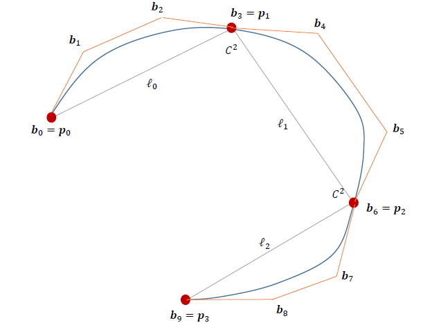
• degree = 3
• 4 points
• Use Bézier end condition.

\[3+1\times3-3-3=4\]

with 4 points

+2 Bessel end conditions

1. Parameterization with chord length

\[P_0 \Rightarrow u_0=0\] \[P_1 \Rightarrow u_1=\|P_1-P_0\|\] \[P_2 \Rightarrow u_2=u_1+\|P_2-P_1\|\] \[P_3 \Rightarrow u_3=u_2+\|P_3-P_2\|\]

1. Apply Bessel end condition

Let

\[x(t)=at^3+bt^2+ct+d, \qquad t\in[0,1]\]

where

\[t=\frac{u-u_0}{u_1-u_0}\] \[\frac{dx(u_0)}{du} = \frac{dx}{dt} \frac{dt}{du} = \frac{1}{u_1-u_0} \frac{dx}{dt} = \frac{3}{l_0}(b_1-b_0)\] \[\frac{dx(u_3)}{du} = \frac{1}{u_3-u_2} \frac{dx}{dt} = \frac{3}{l_2}(b_3-b_2)\]

Apply POC condition, continuity at junction point.

\[X'(u_1^-)=X'(u_1^+)\] \[X''(u_1^-)=X''(u_1^+)\] \[\frac{3}{l_0}(b_3-b_2) = \frac{3}{l_1}(b_4-b_3)\] \[\frac{3\cdot2}{l_0^2}(b_3-2b_2+b_1) = \frac{3\cdot2}{l_1^2}(b_5-2b_4+b_3)\] \[X'(u_2^-)=X'(u_2^+)\] \[X''(u_2^-)=X''(u_2^+)\] \[\frac{3}{l_1}(b_6-b_5) = \frac{3}{l_2}(b_7-b_6)\] \[\frac{3\cdot2}{l_1^2}(b_6-2b_5+b_4) = \frac{3\cdot2}{l_2^2}(b_8-2b_7+b_6)\] \[X(u_0)=P_0=b_0\] \[X(u_1)=P_1=b_3\] \[X(u_2)=P_2=b_6\] \[X(u_3)=P_3=b_9\] \[A \begin{bmatrix} b_1\\ b_2\\ b_4\\ b_5\\ b_7\\ b_8 \end{bmatrix} = \begin{bmatrix} \cdots \end{bmatrix}\]

---

2. Interpolation (Global) / One Polynomial

\[t=\frac{u-a}{b-a}, \qquad u\in[a,b]\]

1. Parameterization with chord length

\[P_0=X(u_0)=b_0B_0^3(0), \qquad u_0=a\] \[P_1=X(u_1) = b_0B_0^3(u_1) +b_1B_1^3(u_1) +b_2B_2^3(u_1) +b_3B_3^3(u_1)\]

Solve $4\times4$ linear system.

---

3. Interpolation (Global) / Piecewise Polynomial

Given

• $N$ data points
• $d$ degree
• $C^c$ continuity

\[(d+1)\times \mathrm{seg} - (c+1)\times(\mathrm{seg}-1) - N = 0\]

• Bézier unknowns: $(d+1)\times\mathrm{seg}$
• Continuity constraints: $(c+1)\times(\mathrm{seg}-1)$
• Data points: $N$

Example

• Given 6 data points
• degree $=3$
• $C^1$ continuity

\[4s-2(s-1)-6=0\] \[2s-4=0\] \[s=2\]

2 segments.

4. Approximation with One Polynomial

Example : # of points = 5

• degree = 3
• one Bézier curve

2 ways

1. Chord-length parameterization

For each data point,

\[e_1^2=\|P_1-X(u_1)\|^2\] \[e_2^2=\|P_2-X(u_2)\|^2\] \[e_3^2=\|P_3-X(u_3)\|^2\]

Total error

\[E=b_1^2+b_2^2+b_3^2 =e_1^2+e_2^2+e_3^2\]

where

\[X(u_i) = b_0B_0^3(u_i) +b_1B_1^3(u_i) +b_2B_2^3(u_i) +b_3B_3^3(u_i)\]

or

\[X(u_i) = b_0B_0^3(u_i) +b_3B_3^3(u_i) +b_1B_1^3(u_i) +b_2B_2^3(u_i)\]

Since the unknowns are the interior control points,

\[\frac{\partial E}{\partial b_1}=0\] \[\frac{\partial E}{\partial b_2}=0\]

Solve

\[A^{T}A\,x=A^{T}b\]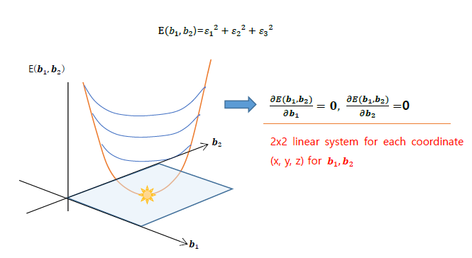

1. Parameterization + Least Squares

Given

• end points fixed
• interior control points unknown

Represent the curve as

\[X(u) = \sum_{i=0}^{3}b_iB_i^3(u)\]

For each data point,

\[P_i\approx X(u_i)\]

Residual

\[r_i=P_i-X(u_i)\]

Objective

\[E=\sum_i\|r_i\|^2\]

Normal equation

\[A^{T}A\,x=A^{T}b\]

7. Polynomial Basis Function

	Monomial	Bernstein	Lagrangian
Function	$f=a_0+a_1t+a_2t^2+\cdots$	$f=\sum B_i^n(t)b_i$	$f=\sum_{i=0}^{n}L_i(t)f_i$
Basis	${1,t,t^2,\ldots}$	$\displaystyle \binom{n}{i}t^i(1-t)^{n-i}$	$\displaystyle L_i(t)=\prod_{j\ne i}\frac{t-t_j}{t_i-t_j}$
Sum-to-one	✗	○	✗
Nonnegativity	✗	○	✗

undefined