[PSA] Chapter 4 - Transmission-Line Modeling

4.1 Derivation of terminal V, I Relations

We can assume that

\[\begin{aligned}z &= r + j\omega l \\ y &=g + j\omega c\end{aligned}\]

where z : series impedance per meter, y : shunt admittance per meter to neutral

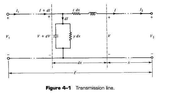
• Applying KVL and KCL, we get

\[\begin{equation}\begin{aligned}dV &= Iz\,dx, \\dI &= (V+dV)y\,dx \approx Vy\,dx\end{aligned}\tag{4.1}\end{equation}\] \[\begin{equation}\begin{aligned}\frac{dV}{dx} &= zI, \\\frac{dI}{dx} &= yV\end{aligned}\tag{4.2}\end{equation}\] \[\begin{equation}\frac{d^{2}V}{dx^{2}}=yzV=\gamma^{2}V\tag{4.3}\end{equation}\] \[\begin{equation}\frac{d^{2}I}{dx^{2}}=yzI=\gamma^{2}I\tag{4.4}\end{equation}\]

• By substituting $I$ into another equation, we can get (4.3) : the second-order differential equation
• $\gamma\triangleq \sqrt{yz}$ : propagation constant. without resistance, its purely imaginary → if not, cannnot expect real solutions for (4.3) or (4.4)
• Applying initial condition, and Boundary condition,

\[\begin{equation}\frac{dV(0)}{dx}=zI_{2}\tag{4.7}\end{equation}\] \[V=V_2 \ (x=0), \ I=I_2 \ (x=0)\]

• we can get

\[\begin{equation}\begin{aligned}V&=V_{2}\cosh(\gamma x)+Z_{c}I_{2}\sinh(\gamma x), \\I&=I_{2}\cosh(\gamma x)+\frac{V_{2}}{Z_{c}}\sinh(\gamma x)\end{aligned}\tag{4.9}\end{equation}\] \[\begin{equation}\begin{aligned}V_{1}&=V_{2}\cosh(\gamma\ell)+Z_{c}I_{2}\sinh(\gamma\ell), \\I_{1}&=I_{2}\cosh(\gamma\ell)+\frac{V_{2}}{Z_{c}}\sinh(\gamma\ell)\end{aligned}\tag{4.10}\end{equation}\]

• $Z_c \triangleq \sqrt{z/y}$ : characteristic impedance (to be substituted in terms of impedance)

Surge Impedence Loaded (SIL)

• When lossless transmission line (i.e. $r=g=0$),

\[Z_c = \sqrt{j\omega l \over j\omega c} = \sqrt{L\over C}\]

• Tranmitted power

\[P_{SIL} = {\vert V_1\vert^2 \over Z_c}\]

• Multiplying by 3, the corresponding three-power power

\[P_{SIL}^{3\phi} = {\vert V_1^{ll}\vert^2 \over Z_c}\]

• where $V_1^{ll}$ : line to line voltage magnitude

---

4.2 Waves on Transmission Lines

• The transmission-line voltage consists of incident wave and reflected wave

Division of propagation constant

\[\gamma=\sqrt{zy}=\alpha+j\beta\]

• $\alpha$: attenuation constant
• $\beta$: phase constant

Incident and reflected voltage waves

The time-domain voltage is written as

\[v(t,x) = \sqrt{2}\operatorname{Re} \left\{ K_1e^{\gamma x}e^{j\omega t} \right\} + \sqrt{2}\operatorname{Re} \left\{ K_2e^{-\gamma x}e^{j\omega t} \right\}\]

or

\[v(t,x)=v_1(t,x)+v_2(t,x)\]

• $v_1(t,x)$ : a wave traveling toward the left $v_2(t,x)$ : a wave traveling toward the right.
• $e^{-\alpha x}$ : attenuation as the wave travels. (can neglect, small in any case)
• The factor involving $\beta x$ : the spatial phase shift.

Wave velocity

For a wave traveling along the line,

\[\omega t-\beta x=\text{constant}\]

• Propagation velocity

\[\frac{dx}{dt} = \frac{\omega}{\beta} = \frac{\omega}{\operatorname{Im}\sqrt{zy}}\]

• In a lossless line, wave velocity is constant

Infinite line

• If infinite line extending, there is no reflected wave.

\[\frac{V}{I}=Z_c\]

• No reflected wave is produced when the terminating impedance equals $Z_c$.
• If not, reflected waves are generated
• Voltage doubles when the wave meets open-circuit (because I = 0)

---

4.3 Transmission Matrix

From equation (4.10),

\[V_1=AV_2+BI_2\] \[I_1=CV_2+DI_2\]

where

• $A=\cosh(\gamma\ell)$, $B=Z_c\sinh(\gamma\ell)$ $C=\frac{1}{Z_c}\sinh(\gamma\ell)$, $D=\cosh(\gamma\ell)$

Transmission matrix

\[\begin{bmatrix} V_1\\ I_1 \end{bmatrix} = \begin{bmatrix} A&B\\ C&D \end{bmatrix} \begin{bmatrix} V_2\\ I_2 \end{bmatrix}\]

• $\mathbf T$ : transmission matrix or chain matrix

\[\mathbf T = \begin{bmatrix} A&B\\ C&D \end{bmatrix}\]

• Determinent of $\mathbf T$ : $\det \mathbf T = 1$

Therefore,

\[\mathbf T^{-1} = \begin{bmatrix} D&-B\\ -C&A \end{bmatrix}\]

Cascaded networks

For cascaded transmission networks can figure composite equivalent transmission matrix by simply multiplying two matrixs with order.

\[\mathbf T=\mathbf T_1\mathbf T_2\]

---

4.4 Lumped-Circuit Equivalent

$\Pi$ - equivalent circuit equations

• A series impedance $Z’$
• Two equal shunt admittances $Y’/2$

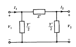
• ABCD parameters of $\Pi$ circuit can be represented with $Z’, Y’/2$
• $A=1+\frac{Z’Y’}{2}$, $B=Z’$, $C=Y’ \left( 1+\frac{Z’Y’}{4} \right)$, $D=1+\frac{Z’Y’}{2}$

Exact equivalent series impedance

• By equating $B$ parameters, can get relationship along $Z =z\ell$ and $Z’$

\[Z' = Z\frac{\sinh(\gamma\ell)}{\gamma\ell}\]

• Series impedance correlation factor : $\sinh(\gamma\ell) \over \gamma \ell$

Exact equivalent shunt admittance

• By equating $A$ parameters, can get relationship along $Y=y\ell$ and $Y’$

\[\frac{Y'}{2} = \frac{Y}{2} \frac{ \tanh(\gamma\ell/2) }{ \gamma\ell/2 }\]

• Shunt admittance correlation factor : $\tanh(\gamma \ell /2 ) \over \gamma \ell /2$

Relations using total line parameters

\[Z_c=\sqrt{\frac{Z}{Y}}\] \[\gamma\ell=\sqrt{ZY}\]

Short-line approximation of correction factors

• $|\gamma\ell|\ll1$, correlations factors are approximately $1$,
• Therefore $Z’ \approx Z, Y’ \approx Y$

---

4.5 Simplified Models

• For a long line (approximately $\ell > 150 \text{ mi}$) → use exact $\Pi$ - equivalent model
• For medium-length line (approx. $50 < \ell < 150 \text { mi}$), use nominal $\Pi$ model)
• For short line (approx. $\ell < 50 \text{ mi}$), neglect shunt admittance($Y\approx 0$)

Nominal $\Pi$ model

• Therefore $Z’ \approx Z=z\ell, Y’ \approx Y = y\ell$

---

4.6 Complex Power Transmission: Short Line

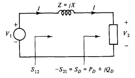
• For short line, model each transmission line with series $RL$ circuit

\[Z=R+j\omega L = |Z|e^{j\theta_Z}\]

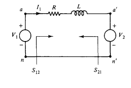
Assume following notations : $V_1=|V_1|e^{j\theta_1}$, $V_2=|V_2|e^{j\theta_2}$, power angle $\theta_{12}=\theta_1-\theta_2$

• Can compute $S_{12}$ and $S_{21}$ with some equations ($S_{12} = V_1I_1^*$, $I_1 = (V_1-V_2)/Z$)

\[S_{12} = \frac{|V_1|^2}{|Z|}e^{j\theta_Z} - \frac{|V_1||V_2|}{|Z|} e^{j(\theta_Z+\theta_{12})}\]

• Similarly,

\[S_{21} = \frac{|V_2|^2}{|Z|}e^{j\theta_Z} - \frac{|V_1||V_2|}{|Z|} e^{j(\theta_Z-\theta_{12})}\]

Power-circle equations

• $Z, V_1, V_2$ are fixed ($Z$ by geometry, voltages are controlled strictly via generators)
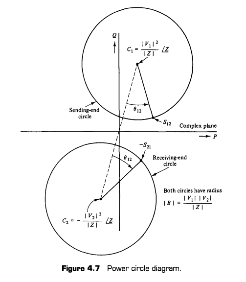
• Can write $S_{12}$, sending-end power circle, $-S_{21}$, receiving-end power circle

\[S_{12}=C_1-Be^{j\theta_{12}}\] \[S_{21}=C_2+Be^{-j\theta_{12}}\]

• with radius

\[B = \frac{|V_1||V_2|}{|Z|}\]

Lossless short line

• For most lines resistance is small compared to inductance. Assume $R\approx 0, Z = jX$

\[P_{12} = -P_{21} = \frac{|V_1||V_2|}{X} \sin\theta_{12}\] \[Q_{12} = \frac{|V_1|^2}{X} - \frac{|V_1||V_2|}{X} \cos\theta_{12}\] \[Q_{21} = \frac{|V_2|^2}{X} - \frac{|V_1||V_2|}{X} \cos\theta_{12}\]

Maximum active-power transmission

• The maximum active power is achieved when $\theta_{12} = 90 ^\circ$for a lossless line

\[P_{\max} = \frac{|V_1||V_2|}{X}\]

Active- and reactive-power control

• Under normal high-voltage operating conditions, we assume $|V_1|\approx|V_2|, \theta_{12}«1$
• In that case, Substituting into previous equation (Lossless)

\[P_{12} = -P_{21} \approx {\vert V_1 \vert \vert V_2\vert \over X}(\theta_{12})\] \[Q_{12} \approx {\vert V_1 \vert \over X}(\vert V_1 \vert - \vert V_2 \vert)\]

• Coupling between active power and power angle / reactive power and voltage magnitude difference.
• Is valid only if small $R$ compared to $X$, small $\theta_{12}$, $\vert V_1 \vert \approx \vert V_2 \vert$, short line

---

4.7 Complex Power Transmission: Short Radial Line

• A radial line has voltage support at the sending end but not at the receiving end.
• The receiving-end load is represented by a fixed power factor.
• At an receiving end, $PF$ is fixed, it “Draws” complex power.

• Load Complex power

\[S_D = V_2I^* = |V_2||I|(\cos\phi+j\sin\phi) = P_D(1+j\beta)\]

• where $\beta=\tan{\phi}$, Positive value if lagging power factor, negative if leading.
• $P_D$: load active power
• $Q_D=\beta P_D$: load reactive power

Power equations for a lossless radial line

• For lossless line, $Z=jX$.

\[P_D = P_{12} = \frac{|V_1||V_2|}{X} \sin\theta_{12}\] \[Q_D = -Q_{21} = -\frac{|V_2|^2}{X} + \frac{|V_1||V_2|}{X} \cos\theta_{12}\] \[Q_D=\beta P_D\]

• Remove power angle with trigonometric identy, gives following eqn\

\[\left( \beta P_D+\frac{|V_2|^2}{X} \right)^2 = \left( \frac{|V_1||V_2|}{X} \right)^2 - P_D^2\]

Receiving-end voltage equation

Rearranging gives a quadratic equation in $|V_2|^2$:

\[|V_2|^4 + \left( 2\beta P_DX-|V_1|^2 \right)|V_2|^2 + (1+\beta^2)P_D^2X^2 = 0\]

The two possible solutions exists :

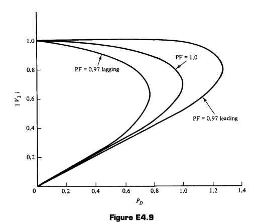
\[|V_2|^2 = \frac{|V_1|^2}{2} - \beta P_DX \pm \left[ \frac{|V_1|^4}{4} - P_DX \left( P_DX+\beta|V_1|^2 \right) \right]^{1/2}\]

• The higher-voltage solution represents the normal operating branch.
• The lower-voltage solution represents an abnormal low-voltage branch.

Voltage-collapse point

• As $P_D$ increases, two solutions approach. When it meets → the limiting condition is called ‘Voltage collapse’.
• At this point, we also call it ‘maximum loadability’

Effect of power factor

• A lagging power factor($\beta>0$) : Reduces the maximum load
• A leading power factor($\beta<0$) : Improves receiving-end voltage , increases loadability.
• Load has capacitive property, supplies reactive power → Aids on sustaining high voltage, can transfer higher real power. → Importance of short transmission line.

---

4.8 Complex Power Transmission: Long or Medium Line

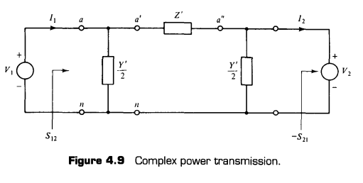
• Must take account into $\Pi$ - transmission line modeling

Sending-end complex power

\[S_{12} = \frac{Y'^*}{2}|V_1|^2 + \frac{|V_1|^2}{Z'^*} - \frac{|V_1||V_2|}{Z'^*} e^{j\theta_{12}}\]

• First term : Power consumed by sending-end shunt admittance
• Remaining terms : Series branch

Receiving-end complex power

\[S_{21} = -\frac{Y'^*}{2}|V_2|^2 - \frac{|V_2|^2}{Z'^*} + \frac{|V_1||V_2|}{Z'^*} e^{-j\theta_{12}}\]

• First term : the receiving-end shunt-admittance contribution.
• Remaining terms : have the same structure as the short-line power equations.

Power-circle interpretation

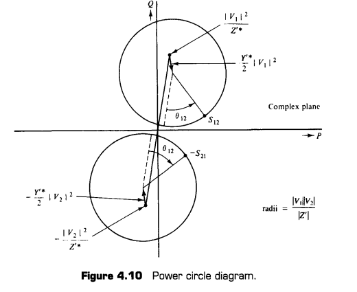
• $Y’$ is almost reactive : so the shift is approximately vertical.
• Short-line model’s general conclusions still remain valid

---

4.9 Power-Handling Capability of Lines

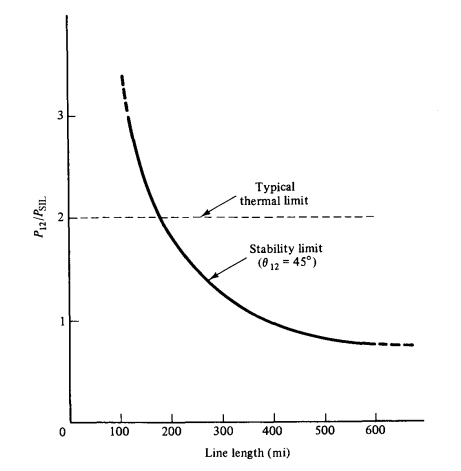
• Thermal, Stability limits transmission-line power capability

Thermal limit

• Real power loss generated by line $P_{\mathrm{loss}}=I^2R$
• It reduces efficiency, raise heat(also stratches due to thermal expansion)

Current rating, Voltage, MVA, MW limitation

• Line current “rating” : condition for certain line to operate at normal condition’
• Voltage limitation also exists
• Limitation on MVA, MW also exists

Stability limit

• Theoretical maximum transfer capability ($\theta_{12} = 90^\circ$) for lossless, short line
• Practically, power angle is limited to $\theta_{12} = 40^\circ\text{ to }50^\circ$. (Approx. $65\%$ to $75\%$ of theoretical maximum)

Lossless long-line equivalent parameters

• Can neglect $\alpha$ in lossless line (i.e. $\gamma=j\beta$)
• Shunt admittance

\[Y' = Y \frac{ \tanh(\gamma\ell/2) }{ \gamma\ell/2 } = j\omega C \frac{ \tan(\beta\ell/2) }{ \beta\ell/2 }\]

• Series impedance

\[Z' = Z \frac{ \sinh(\gamma\ell) }{ \gamma\ell } = j\omega L \frac{ \sin(\beta\ell) }{ \beta\ell } = jZ_c\sin(\beta\ell)\]

Active power of a lossless long line

• Equal voltage magnitudes, at both ends : $|V_1|=|V_2|$
• Transmitted active power :

\[P_{12} = -P_{21} = \frac{|V_1|^2} {Z_c\sin(\beta\ell)} \sin\theta_{12}\]

• Applying results to surge-impedance loading,

\[P_{12} = P_{\mathrm{SIL}} \frac{ \sin\theta_{12} }{ \sin(\beta\ell) }\]

• Interpretation : for fixed power angle, the maximum transferable power decreases as line length increases.
• Applied both stability and thermal limitations