[PSA] Chapter 3 - Transmission-line parameters

3.0 Introduction

• A transmission line is characterized by distributed $R, L, G,C.$ : Series / Shunt
• Inductance and capacitance result from magnetic and electric fields.
• Shunt conductance represents leakage and is often neglected.

3.1 Review of Magnetics

Ampere’s circuital law

\[\oint_\Gamma {\mathbf H}\cdot d{\mathbf l} = i_ℓ\]

• $\mathbf H$: magnetic field intensity
• $d\mathbf l$: along path
• $i_ℓ$: total instantaneous current enclosing closed path
• follows right hand rule

Magnatic flux density and magntic flux

\[\mathbf B = \mu \mathbf H\]

• $\mu$ : permeability
• Definition of magnatic flux : $\phi = \int_A \mathbf B \cdot da$

Flux linkages

• If every flux penetrates $N$ turns, flux linkage $\lambda = N\phi$

Inductance

• Inductance is defined by the linear relation $\lambda = Li$
• Inductance works as a linear constant between flux linkage and current
• Eg) inductance derivation of toriduial inductor (use simple physics)

\[\begin{aligned}F& =Hl = ni \\ B &= \mu H = \mu {Ni\over l} \\ \phi &= BA = {\mu A \over l}Ni = {NI \over l/\mu A} \\ L &= {\lambda \over i} = {N\phi \over i} = {\mu A N^2 \over 2\pi R} \end{aligned}\]

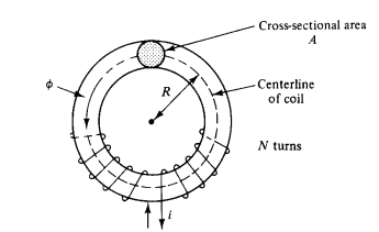
3.2 Flux Linkages of Infinite Straight Wire

• Assume an infinitely long straight conductor with radius $r$.
• The total current is $i$, and the current density is assumed to be uniform.
• The magnetic flux lines are concentric circles around the conductor.

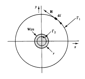
Magnetic field outside the conductor

For $x>r$, the entire conductor current is enclosed.

\[H(2\pi x)=i\] \[H=\frac{i}{2\pi x}\]

Magnetic field inside the conductor

For $x<r$, only part of the current is enclosed.

\[i_\ell=\frac{x^2}{r^2}i\] \[H=\frac{x}{2\pi r^2}i\]

Magnetic flux density

\[B=\mu_0\mu_r H\]

• $\mu_0$: permeability of free space
• $\mu_r$: relative permeability of the conductor
• Outside the conductor, $\mu_r\approx1$ because the surrounding medium is air.
• Recall : Linear inside / inverse proportional outside the wire

External flux linkages

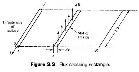
The flux linkages between the conductor surface $r$ and an external radius $R$ are

\[\lambda_{\mathrm{ext}} = \frac{\mu_0 i}{2\pi} \ln\left(\frac{R}{r}\right)\]

• All external flux links the entire conductor current.
• Therefore, external flux and external flux linkage have the same numerical value.

Internal flux linkages

The flux inside the conductor links only a fraction of the total current.

\[\lambda_{\mathrm{int}} = \frac{\mu_0\mu_r i}{8\pi}\]

• Internal flux linkage is independent of the conductor radius under the assumption of uniform current density.

Total flux linkages

\[\lambda = \frac{\mu_0 i}{2\pi} \left[ \frac{\mu_r}{4} + \ln\left(\frac{R}{r}\right) \right]\]

or

\[\lambda = 2\times10^{-7}i \left[ \frac{\mu_r}{4} + \ln\left(\frac{R}{r}\right) \right]\]

• For a single isolated infinite conductor, $\lambda$ increases without bound as $R\rightarrow\infty$.
• This problem is resolved by considering a complete multiconductor transmission line.

---

3.3 Flux Linkages: Many-Conductor Case

• Consider $n$ conductors carrying currents $i_1,i_2,\ldots,i_n$.
• The total flux linkage of one conductor is found using superposition.
• The magnetic field produced by every conductor contributes to the flux linkage of the other conductors.

Zero-sum current condition

For normal transmission-line operation,

\[i_1+i_2+\cdots+i_n=0\]

• Some conductors act as return paths for the currents in the other conductors.
• This condition makes the total flux linkage finite even when the external reference radius approaches infinity.

Equivalent conductor radius

The internal flux linkage can be included in the external flux expression by defining

\[r'=r e^{-\mu_r/4}\]

For a nonmagnetic conductor, $\mu_r=1$:

\[r'=re^{-1/4}=0.7788r\]

• $r’$ is the radius of an equivalent hollow conductor.
• The equivalent hollow conductor has no internal flux but has the same total flux linkage as the original solid conductor.

General flux-linkage equation

For conductor $1$,

\[\lambda_1 = \frac{\mu_0}{2\pi} \left[ i_1\ln\left(\frac{1}{r'_1}\right) + i_2\ln\left(\frac{1}{d_{12}}\right) +\cdots+ i_n\ln\left(\frac{1}{d_{1n}}\right) \right]\]

• $r’_1$: equivalent radius of conductor $1$
• $d_{1k}$: distance between conductor $1$ and conductor $k$
• The flux linkage of one conductor generally depends on all conductor currents.
• Therefore, the general circuit model includes mutual inductance.

Equilaterally spaced three-phase line

Assume

• Equal conductor radii
• Equal phase spacing $D$
• $i_a+i_b+i_c=0$

Then

\[\lambda_a = \frac{\mu_0}{2\pi} i_a\ln\left(\frac{D}{r'}\right)\]

The inductance per phase per meter is

\[l = \frac{\lambda_a}{i_a} = \frac{\mu_0}{2\pi} \ln\left(\frac{D}{r'}\right)\] \[l = 2\times10^{-7} \ln\left(\frac{D}{r'}\right) \quad \mathrm{H/m}\]

• Although physical magnetic coupling exists between phases, the mutual terms disappear under equal spacing and zero-sum current conditions.
• The line can therefore be represented using equal phase self-inductances.
• This result permits per-phase analysis.

---

3.4 Conductor Bundling

• A bundled conductor consists of multiple closely spaced subconductors used for one phase.
• The subconductors are connected by conducting frames and operate electrically in parallel.
• Two, three, or four subconductors per phase are commonly used.
• Bundle spacing is assumed to be much smaller than phase spacing.

Equal current sharing

If a phase contains $b$ identical subconductors, the phase current is assumed to divide equally:

\[i_{\mathrm{sub}} = \frac{i_{\mathrm{phase}}}{b}\]

Bundle geometric mean radius

For $b$ symmetrically arranged subconductors,

\[R_b = \left( r'd_{12}d_{13}\cdots d_{1b} \right)^{1/b}\]

• $R_b$: geometric mean radius, GMR, of the bundle
• $r’$: equivalent radius of one subconductor
• $d_{1k}$: spacing between subconductor $1$ and subconductor $k$

For one conductor per phase,

\[R_b=r'\]

Inductance of a bundled three-phase line

For equal phase spacing $D$,

\[l = \frac{\mu_0}{2\pi} \ln\left(\frac{D}{R_b}\right)\] \[l = 2\times10^{-7} \ln\left(\frac{D}{R_b}\right) \quad \mathrm{H/m}\]

• Bundling replaces the small conductor radius $r’$ with the larger bundle GMR $R_b$.
• Therefore, conductor bundling reduces line inductance.

Additional effects of bundling

• A bundle behaves approximately like a large hollow conductor.
• The increased effective radius reduces the electric field strength at the conductor surface.
• Reduced surface electric field decreases corona, line losses, radio interference, and audible noise.
• Bundled conductors have a larger surface area exposed to air.
• Improved cooling permits greater current without exceeding thermal limits.

---

3.5 Transposition

• Equal triangular phase spacing is not always practical.
• Transmission-line conductors are commonly arranged horizontally or vertically.
• Unequal phase spacing produces unequal phase flux linkages and unequal phase inductances.

Definition of transposition

• Transposition exchanges the physical positions of the three phase conductors along the line.

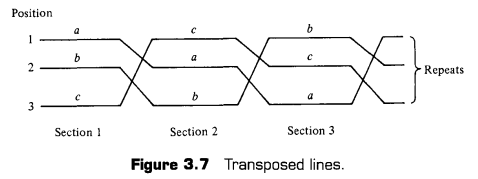
• Equivalent length occupied by each phase and experiences the same average geometric condition.

Geometric mean distance

If the distances between the three physical positions are $d_{12}$, $d_{23}$, and $d_{31}$,

\[D_m = \left( d_{12}d_{23}d_{31} \right)^{1/3}\]

• $D_m$ is the geometric mean distance, GMD, between phases.

Average inductance of a transposed line

For one conductor per phase,

\[\bar l = \frac{\mu_0}{2\pi} \ln\left(\frac{D_m}{r'}\right)\]

For bundled conductors,

\[\bar l = \frac{\mu_0}{2\pi} \ln\left(\frac{D_m}{R_b}\right)\] \[\bar l = 2\times10^{-7} \ln\left(\frac{D_m}{R_b}\right) \quad \mathrm{H/m}\]

• Transposition makes the average inductances of the three phases equal:

\[\bar l_a=\bar l_b=\bar l_c\]

• The result is consistent with per-phase analysis.
• Even when a practical line is not completely transposed, it is often calculated as if it were transposed with little error.
• For stranded conductors, the conductor GMR given by manufacturers is used instead of $r’$.

---

3.6 Impedance of Three-Phase Lines Including Ground Return

• Balanced operation cannot always be assumed.
• Unbalance may result from incomplete transposition, unbalanced loads, or faults.
• During a phase-to-ground fault, current may flow through a neutral conductor and through the earth.
• The effect of neutral and earth-return currents must therefore be included in the line impedance.

General impedance matrix

\[\begin{bmatrix} V_a\\ V_b\\ V_c\\ V_n \end{bmatrix} = \begin{bmatrix} Z_{aa}&Z_{ab}&Z_{ac}&Z_{an}\\ Z_{ba}&Z_{bb}&Z_{bc}&Z_{bn}\\ Z_{ca}&Z_{cb}&Z_{cc}&Z_{cn}\\ Z_{na}&Z_{nb}&Z_{nc}&Z_{nn} \end{bmatrix} \begin{bmatrix} I_a\\ I_b\\ I_c\\ I_n \end{bmatrix}\]

• $Z_{ii}$: self-impedance of conductor $i$
• $Z_{ij}$: mutual impedance between conductors $i$ and $j$
• The impedances include the effect of earth return.

Self-impedance per meter

\[z_{ii} = (r_i+r_d) + j\omega 2\times10^{-7} \ln\left(\frac{D_e}{\mathrm{GMR}_i}\right)\]

• $r_i$: conductor resistance per meter
• $r_d$: earth-return resistance per meter
• $\mathrm{GMR}_i$: GMR of conductor $i$

Mutual impedance per meter

\[z_{ij} = r_d + j\omega 2\times10^{-7} \ln\left(\frac{D_e}{d_{ij}}\right)\]

• $d_{ij}$: distance between conductors $i$ and $j$

Earth-return parameters

\[r_d = 9.869\times10^{-7}f \quad \Omega/\mathrm{m}\] \[D_e = 658.368\sqrt{\frac{\rho}{f}} \quad \mathrm{m}\]

• $f$: operating frequency
• $\rho$: earth resistivity in $\Omega\cdot\mathrm{m}$

If earth resistivity is unknown, the book commonly assumes

\[\rho=100\ \Omega\cdot\mathrm{m}\]

Total line impedance

For a line of length $\ell$,

\[Z_{ij}=z_{ij}\ell\]

Open-circuited neutral

If

\[I_n=0\]

the neutral row and column can be removed from the impedance equation.

Zero neutral voltage

If

\[V_n=0\]

then the neutral current can be eliminated from the equations.

The reduced phase impedances are

\[Z'_{ii} = Z_{ii} - \frac{Z_{in}Z_{ni}}{Z_{nn}}\] \[Z'_{ij} = Z_{ij} - \frac{Z_{in}Z_{nj}}{Z_{nn}}\]

• The balanced, completely transposed line model is a special case of this general impedance model.

---

3.7 Review of Electric Fields

Gauss’s law

\[\oint_A \mathbf D\cdot d\mathbf a=q_\ell\]

• $\mathbf D$: electric flux density
• $d\mathbf a$: differential outward-normal area vector
• $q_\ell$: algebraic sum of charges enclosed by the closed surface
• Gauss’s law is useful when the electric-field geometry has symmetry.

Electric flux density of an infinite line charge

For an infinite conductor with charge $q$ coulombs per meter, choose a cylindrical Gaussian surface of radius $R$ and length $h$.

\[D(2\pi Rh)=qh\]

Therefore,

\[D=\frac{q}{2\pi R}\]

In vector form,

\[\mathbf D = \frac{q}{2\pi R}\mathbf a_R\]

• The electric flux density is directed radially away from a positive line charge.

Electric field intensity

\[\mathbf D=\epsilon\mathbf E\] \[\mathbf E=\frac{\mathbf D}{\epsilon}\]

• $\epsilon$: permittivity of the medium

In free space,

\[\epsilon=\epsilon_0 = 8.854\times10^{-12}\ \mathrm{F/m}\]

• For dry air, the relative permittivity is approximately $1$.

Voltage difference

The voltage difference between points $P_a$ and $P_b$ is

\[V_{ba} = V_b-V_a = -\int_{P_a}^{P_b}\mathbf E\cdot d\mathbf l\]

---

3.8 Line Capacitance

• Capacitance relates conductor charge to conductor voltage.
• The electric field of an infinite line charge is used to calculate the voltage between points.

Voltage produced by one infinite line charge

For two points at radial distances $R_a$ and $R_b$,

\[V_b-V_a = \frac{q}{2\pi\epsilon} \ln\left(\frac{R_a}{R_b}\right)\]

• A point closer to a positive conductor has a higher potential.
• For one isolated conductor, voltage relative to infinity is not finite.
• A finite result is obtained for a multiconductor line when the total charge is zero.

Zero-sum charge condition

\[q_1+q_2+\cdots+q_n=0\]

• This condition is analogous to the zero-sum current condition used in the inductance derivation.

Voltage of conductor $1$

\[v_1 = \frac{1}{2\pi\epsilon} \left[ q_1\ln\left(\frac{1}{r_1}\right) + q_2\ln\left(\frac{1}{d_{12}}\right) +\cdots+ q_n\ln\left(\frac{1}{d_{1n}}\right) \right]\]

• $r_1$: actual radius of conductor $1$
• $d_{1k}$: distance between conductors $1$ and $k$
• Unlike inductance calculations, capacitance calculations use the actual radius $r$, not $r’$.

Capacitance matrix

\[\mathbf v=\mathbf F\mathbf q\]

The inverse relationship is

\[\mathbf q=\mathbf C\mathbf v\] \[\mathbf C=\mathbf F^{-1}\]

• In the general multiconductor case, mutual capacitances exist.
• Conductor charges depend on all conductor voltages.

Equilaterally spaced three-phase line

Assume equal conductor radii, equal phase spacing $D$, and

\[q_a+q_b+q_c=0\]

Then the phase-to-neutral capacitance per meter is

\[c = \frac{2\pi\epsilon} {\ln(D/r)} \quad \mathrm{F/m\ to\ neutral}\]

Transposed bundled three-phase line

\[c = \frac{2\pi\epsilon} {\ln(D_m/R_b^c)} \quad \mathrm{F/m\ to\ neutral}\]

The bundle radius for capacitance is

\[R_b^c = \left( r d_{12}d_{13}\cdots d_{1b} \right)^{1/b}\]

• $R_b^c$ uses the actual subconductor radius $r$.
• The inductance bundle GMR $R_b$ uses $r’$.

Without bundling,

\[R_b^c=r\]

Capacitive susceptance and reactance

\[B_c=\omega c\] \[X_c=\frac{1}{\omega c}\]

• The effect of the conducting earth is neglected in this derivation.
• For transmission lines at reasonable heights under normal operating conditions, the earth effect is usually small.

---

3.9 Determination of Line Parameters Using Tables

• Manufacturer tables provide conductor resistance, GMR, inductive reactance, and capacitive reactance.
• The appendix tables use inches, feet, and miles.
• In practical line analysis, reactance values are often used directly instead of inductance and capacitance values.

Inductive reactance per phase

For a transposed line with one conductor per phase,

\[X_L = 2.022\times10^{-3}f \ln\left(\frac{D_m}{\mathrm{GMR}}\right) \quad \Omega/\mathrm{mi}\]

The expression can be divided into two terms:

\[X_L=X_a+X_d\] \[X_a = 2.022\times10^{-3}f \ln\left(\frac{1}{\mathrm{GMR}}\right)\] \[X_d = 2.022\times10^{-3}f\ln(D_m)\]

• $X_a$: inductive reactance at $1$ft spacing
• $X_a$ depends on frequency and conductor GMR.
• $X_d$: inductive reactance spacing factor
• $X_d$ depends on frequency and phase spacing.
• $X_d$ is independent of conductor type.

Capacitive reactance to neutral

\[X_C = \frac{1}{2\pi f c} \quad \Omega\cdot\mathrm{mi\ to\ neutral}\]

For one conductor per phase,

\[X_C = \frac{1.779\times10^6}{f} \ln\left(\frac{D_m}{r}\right) \quad \Omega\cdot\mathrm{mi\ to\ neutral}\]

This can also be divided into a conductor term and a spacing term:

\[X_C=X'_a+X'_d\]

• $X’_a$ depends on the conductor radius.
• $X’_d$ depends on the spacing between phases.
• The terms can be obtained directly from the appendix tables.

---

3.10 Typical Parameter Values

• Typical data are provided for $138$kV, $345$kV, and $765$kV transmission lines.

Phase spacing and bundling

• Phase spacing increases as the line-voltage rating increases.
• The number of subconductors per phase also increases with voltage rating.
• The larger bundle GMR causes inductance to decrease even though phase spacing increases.

Resistance

• Line resistance increases with temperature.
• Line resistance also increases with frequency.
• At dc, current density is approximately uniform over the conductor cross section.
• At higher frequency, current density becomes greater near the conductor surface.
• This effect increases $I^2R$ losses and effective resistance.
• The resistance at $60$ Hz in the given table is approximately $5\%$ higher than the dc resistance.

Resistance compared with reactance

• Line resistance is relatively small compared with inductive reactance.
• Resistance may sometimes be neglected in calculations of power flow, voltage, and current.
• Resistance remains important in calculations of line losses, thermal limits, and economic operation.

Surge impedance loading

• Surge impedance loading is listed as a measure of the line power-handling capability.
• It is discussed further in Chapter 4.

Ground wires

• Ground wires are installed above the phase conductors.
• They are electrically connected to ground or to each transmission tower.
• They shield the phase conductors from lightning strikes.
• They also provide a low-impedance path during a phase-to-ground fault.

---

3.11 Summary

Average inductance of a transposed bundled line

\[l = \frac{\mu_0}{2\pi} \ln\left(\frac{D_m}{R_b}\right)\] \[l = 2\times10^{-7} \ln\left(\frac{D_m}{R_b}\right) \quad \mathrm{H/m}\]

where

\[D_m = \left( d_{ab}d_{bc}d_{ca} \right)^{1/3}\]

and

\[R_b = \left( r'd_{12}d_{13}\cdots d_{1b} \right)^{1/b}\]

Without bundling,

\[R_b=r'\]

Average capacitance to neutral

\[c = \frac{2\pi\epsilon} {\ln(D_m/R_b^c)} \quad \mathrm{F/m\ to\ neutral}\]

where

\[R_b^c = \left( r d_{12}d_{13}\cdots d_{1b} \right)^{1/b}\]

Without bundling,

\[R_b^c=r\]

Main geometric relationships

• Increasing $D_m$ increases inductance.
• Increasing $D_m$ decreases capacitance.
• Increasing bundle radius decreases inductance.
• Increasing bundle radius increases capacitance.
• Inductance and capacitance therefore have approximately inverse geometric relationships.
• Ground-return effects are included using Carson’s impedance approach.
• Inductive and capacitive reactances can also be calculated using conductor tables.