LN08. Coons Patch

2. Coons Patch

• Input: 4 boundary curves
• Output: one surface with the given 4 boundary curves

For two opposite boundary curves $\mathbf{b}(u)$ and $\mathbf{c}(u)$,

\[\mathbf{S}_1(u,v)=(1-v)\mathbf{b}(u)+v\mathbf{c}(u)\]

For the other two boundary curves $\mathbf{a}(v)$ and $\mathbf{d}(v)$,

\[\mathbf{S}_2(u,v)=(1-u)\mathbf{a}(v)+u\mathbf{d}(v)\]

Bilinear patch

\[\mathbf{S}_{12}(u,v) =(1-u)(1-v)\mathbf{p}_{00} +u(1-v)\mathbf{p}_{10} +(1-u)v\mathbf{p}_{01} +uv\mathbf{p}_{11}\]

Coons patch

\[\mathbf{S}(u,v)=\mathbf{S}_1(u,v)+\mathbf{S}_2(u,v)-\mathbf{S}_{12}(u,v)\]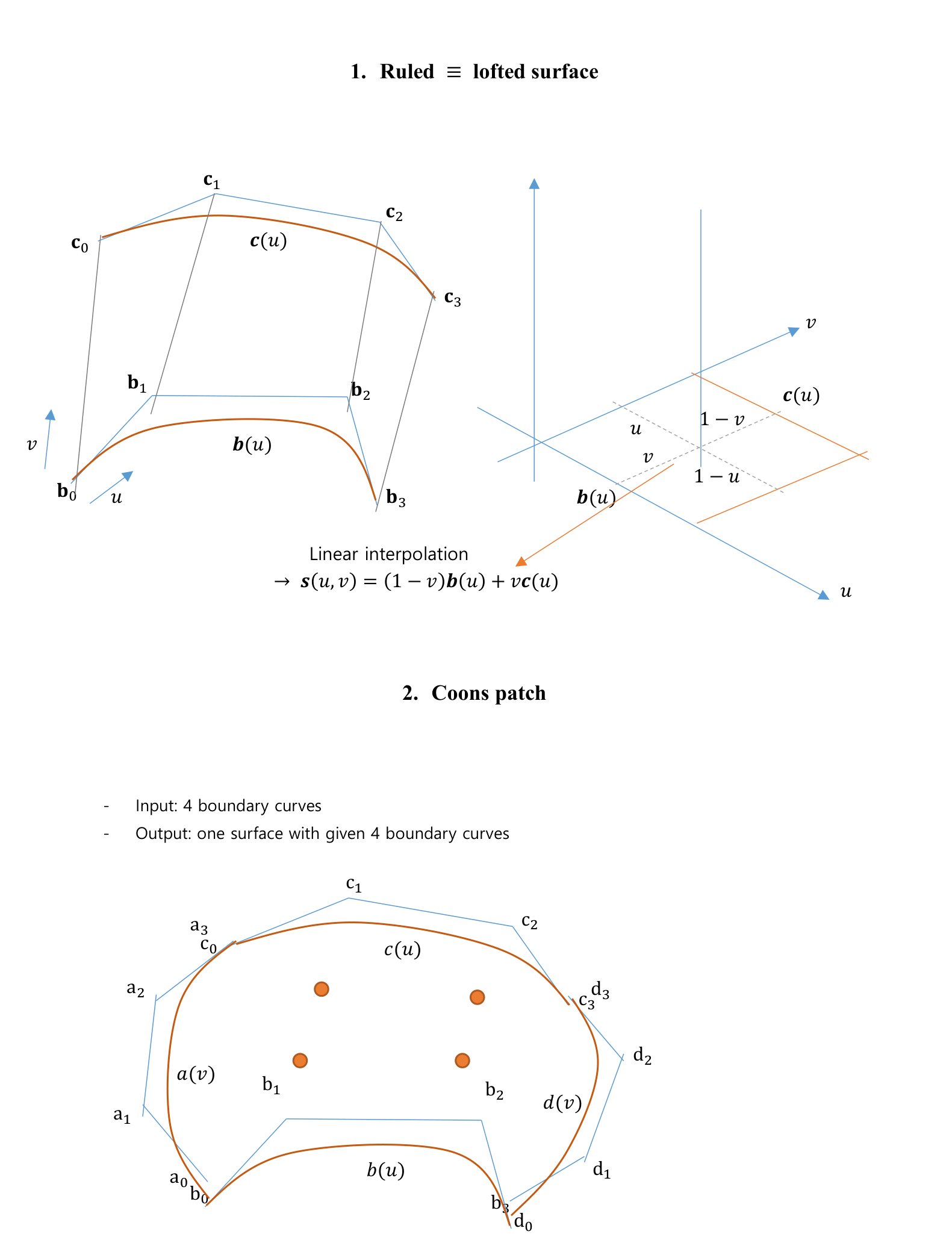

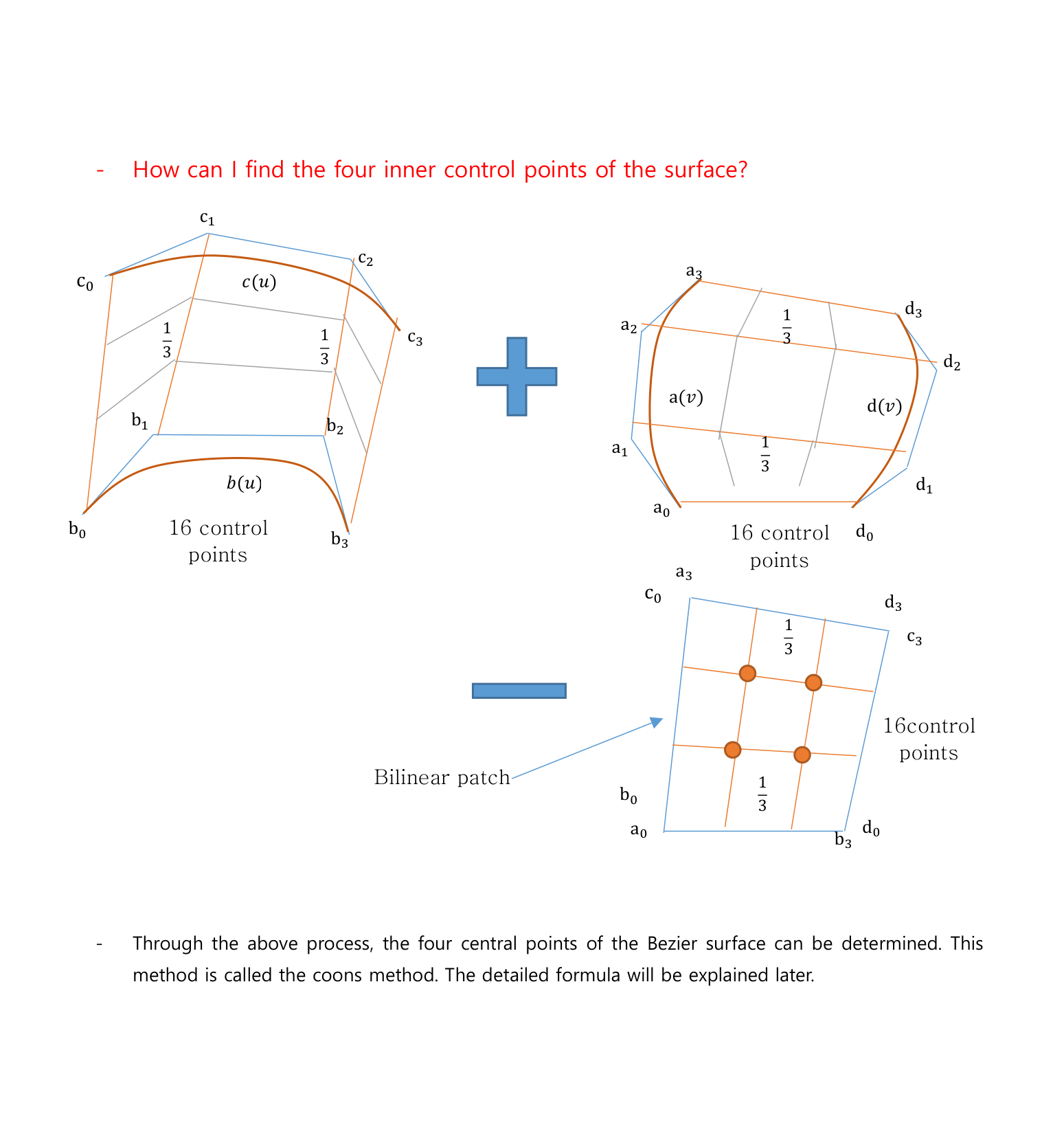
• Find the four inner control points of the surface.
• Add the two ruled surfaces and subtract the bilinear patch.

3. Bézier Surface - Degree Elevation

If a linear boundary in the $v$ direction is elevated to degree 3,

\[\mathbf{b}_{11}=\frac{2}{3}\mathbf{b}_{10}+\frac{1}{3}\mathbf{b}_{13}\] \[\mathbf{b}_{12}=\frac{1}{3}\mathbf{b}_{10}+\frac{2}{3}\mathbf{b}_{13}\] \[\mathbf{b}_{21}=\frac{2}{3}\mathbf{b}_{20}+\frac{1}{3}\mathbf{b}_{23}\] \[\mathbf{b}_{22}=\frac{1}{3}\mathbf{b}_{20}+\frac{2}{3}\mathbf{b}_{23}\]

For the bilinear patch,

\[\begin{aligned} \mathbf{b}_{11} &=\left(\frac{2}{3}\mathbf{b}_{00}+\frac{1}{3}\mathbf{b}_{30}\right)\frac{2}{3} +\frac{1}{3}\left(\frac{2}{3}\mathbf{b}_{03}+\frac{1}{3}\mathbf{b}_{33}\right)\\ &=\frac{4}{9}\mathbf{b}_{00} +\frac{2}{9}\mathbf{b}_{30} +\frac{2}{9}\mathbf{b}_{03} +\frac{1}{9}\mathbf{b}_{33} \end{aligned}\]

• If the boundary degrees do not match, elevate the degree.
• The representation changes, but the surface remains the same.

4. Triangular Bézier Surface

Triangular Bernstein basis

\[B_{ijk}^{n}(u,v,w) =\frac{n!}{i!j!k!}u^iv^jw^k, \qquad i+j+k=n\]

Triangular Bézier surface

\[\mathbf{S}(u,v,w) =\sum_{i+j+k=n}\mathbf{b}_{ijk}B_{ijk}^{n}(u,v,w)\]

5. Barycentric Coordinate

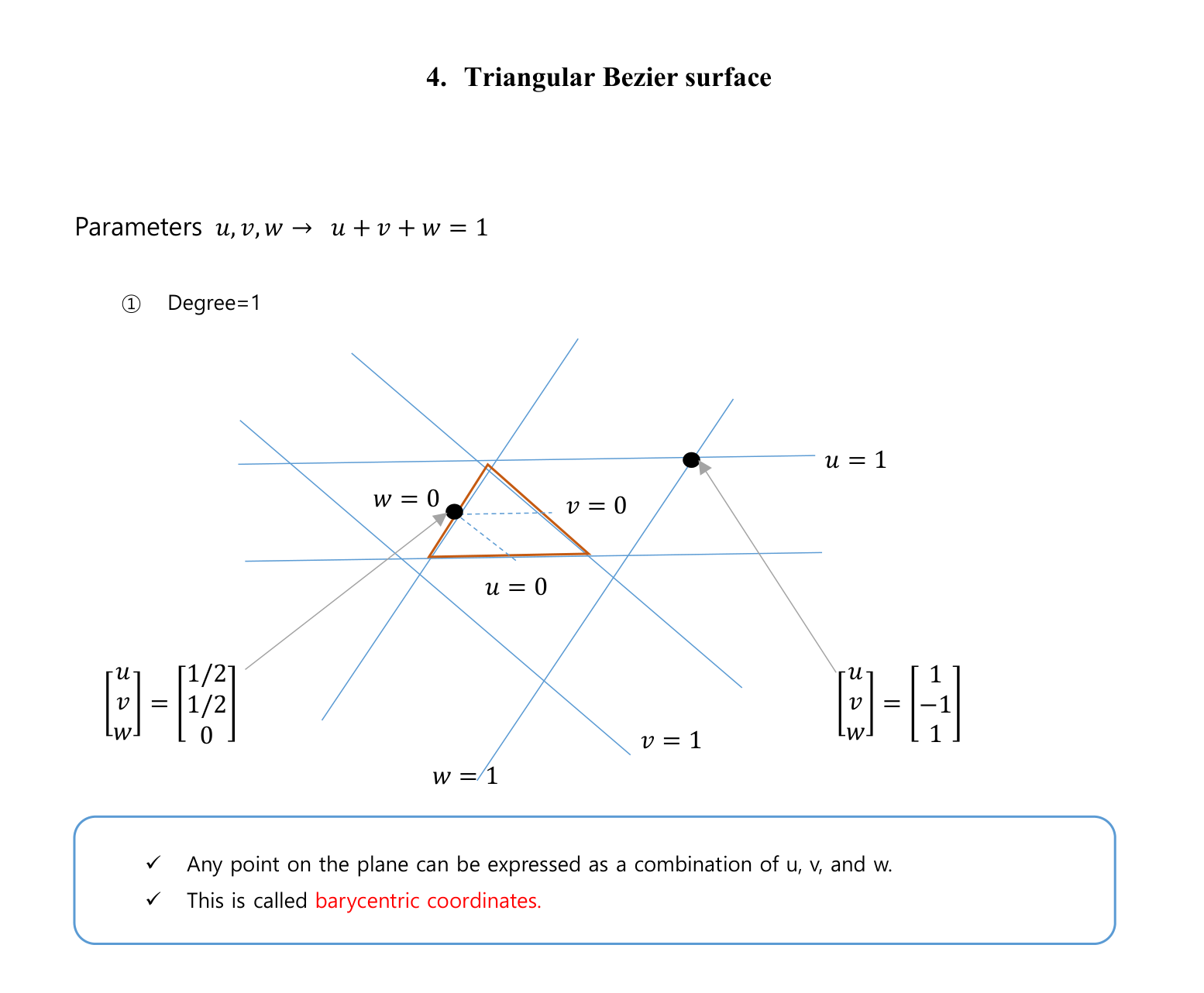
Parameters

\[u+v+w=1\]

• $u=1$, $v=1$, and $w=1$ correspond to the three vertices.
• $u=0$, $v=0$, and $w=0$ correspond to the three opposite edges.
• Any point on the plane of the triangle can be represented using $u$, $v$, and $w$.

\[\mathbf{p}=u\mathbf{b}_0+v\mathbf{b}_1+w\mathbf{b}_2\]

6. Triangular Coons Patch

• Input: 3 boundary curves
• Output: one surface with the given 3 boundary curves
• Find the center control point automatically.

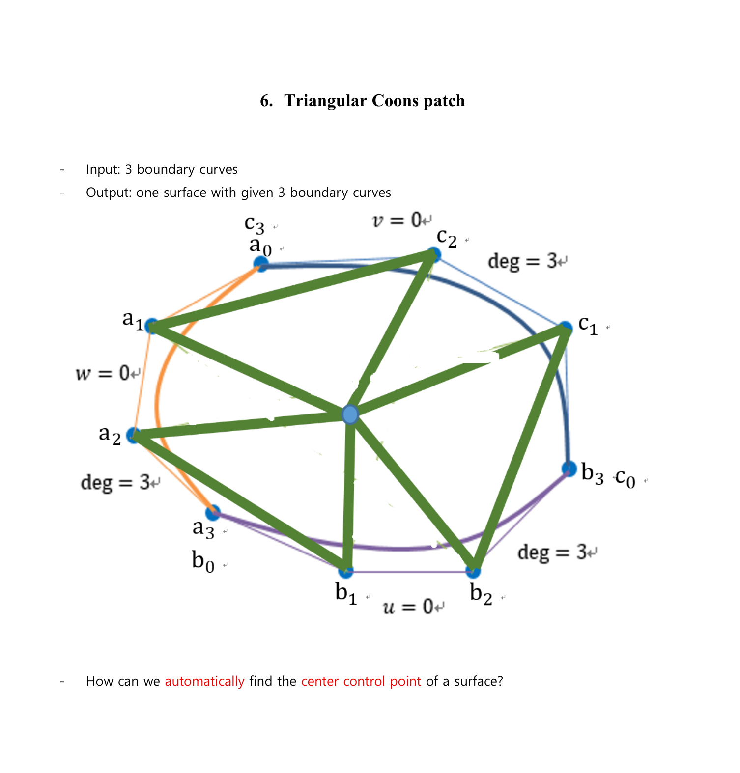
The triangular Coons patch is obtained by adding three directional patches and subtracting the linear triangular patch.

\[\mathbf{S}(u,v,w) =\frac{1}{2} \left( \mathbf{S}_{u} +\mathbf{S}_{v} +\mathbf{S}_{w} -\mathbf{S}_{L} \right)\]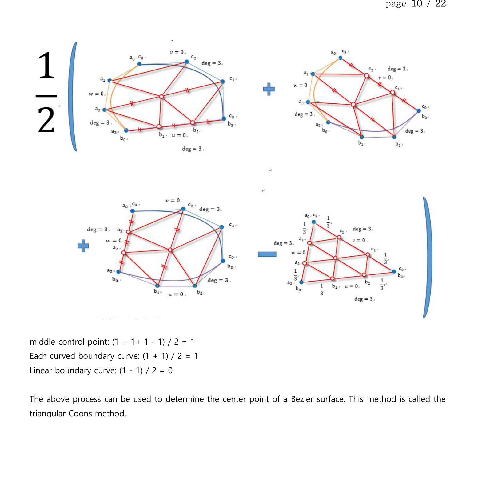

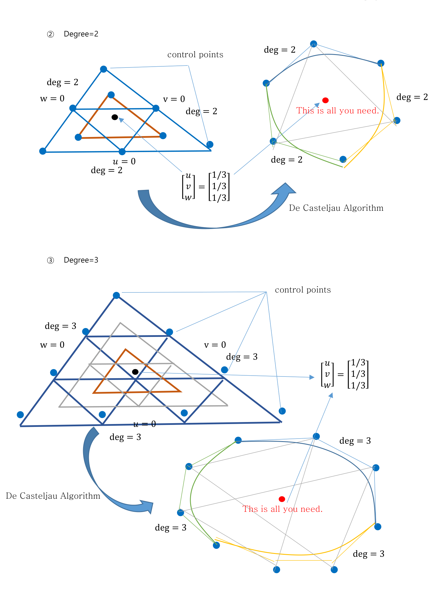
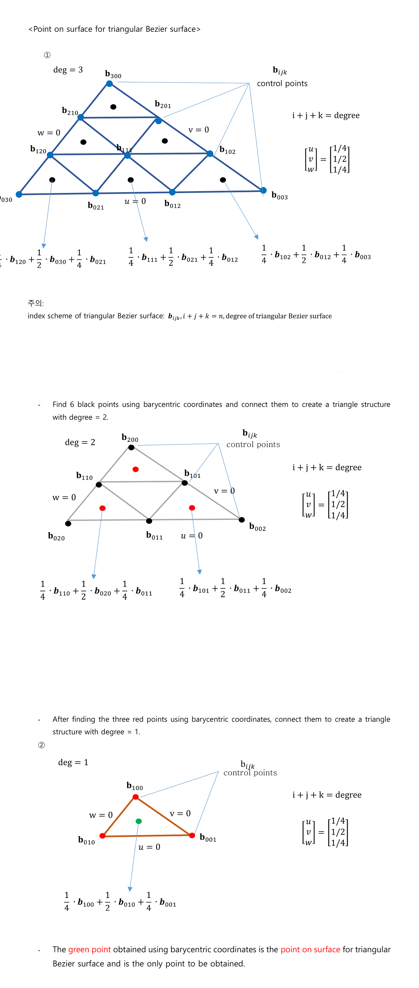
\[\text{middle control point}:\quad \frac{1+1+1-1}{2}=1\] \[\text{each curved boundary point}:\quad \frac{1+1}{2}=1\] \[\text{linear-boundary point}:\quad \frac{1-1}{2}=0\]

7. De Casteljau Algorithm for Triangular Bézier Surface

At each step, form a new control point from three neighboring control points.

\[\mathbf{b}_{ijk}^{(r)} =u\mathbf{b}_{i+1,j,k}^{(r-1)} +v\mathbf{b}_{i,j+1,k}^{(r-1)} +w\mathbf{b}_{i,j,k+1}^{(r-1)}\]

where

\[i+j+k=n-r\]

• Apply the weighted average.
• Reduce the degree by 1.
• Repeat until one point remains.

\[\operatorname{PoS}=\mathbf{b}_{000}^{(n)}\]

8. Degree Elevation

For one degree elevation of a degree-$n$ Bézier curve,

\[\mathbf{b}_{i}^{(1)} =\frac{i}{n+1}\mathbf{b}_{i-1} +\frac{n+1-i}{n+1}\mathbf{b}_{i}\]

For a cubic Bézier curve,

\[\mathbf{x}(t) =\mathbf{b}_{0}B_{0}^{3}(t) +\mathbf{b}_{1}B_{1}^{3}(t) +\mathbf{b}_{2}B_{2}^{3}(t) +\mathbf{b}_{3}B_{3}^{3}(t)\]

Multiply by the sum-to-one term.

\[t+(1-t)=1\]

Then

\[\begin{aligned} \mathbf{x}(t) ={}&\mathbf{b}_{0}(1-t)^4 +\frac{\mathbf{b}_{0}+3\mathbf{b}_{1}}{4}\,4(1-t)^3t\\ &+\frac{3\mathbf{b}_{1}+3\mathbf{b}_{2}}{6}\,6(1-t)^2t^2\\ &+\frac{3\mathbf{b}_{2}+\mathbf{b}_{3}}{4}\,4(1-t)t^3 +\mathbf{b}_{3}t^4 \end{aligned}\]

Therefore,

\[\mathbf{b}_{0}^{(1)}=\mathbf{b}_{0}\] \[\mathbf{b}_{1}^{(1)}=\frac{\mathbf{b}_{0}+3\mathbf{b}_{1}}{4}\] \[\mathbf{b}_{2}^{(1)}=\frac{\mathbf{b}_{1}+\mathbf{b}_{2}}{2}\] \[\mathbf{b}_{3}^{(1)}=\frac{3\mathbf{b}_{2}+\mathbf{b}_{3}}{4}\] \[\mathbf{b}_{4}^{(1)}=\mathbf{b}_{3}\]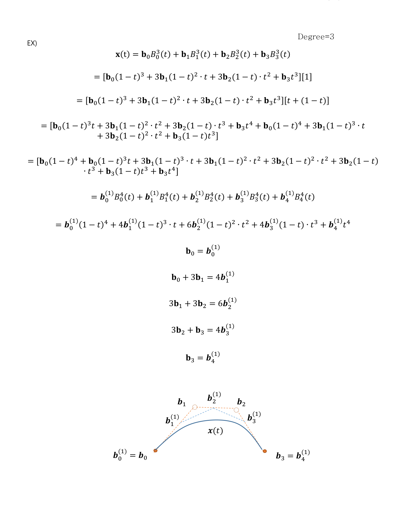

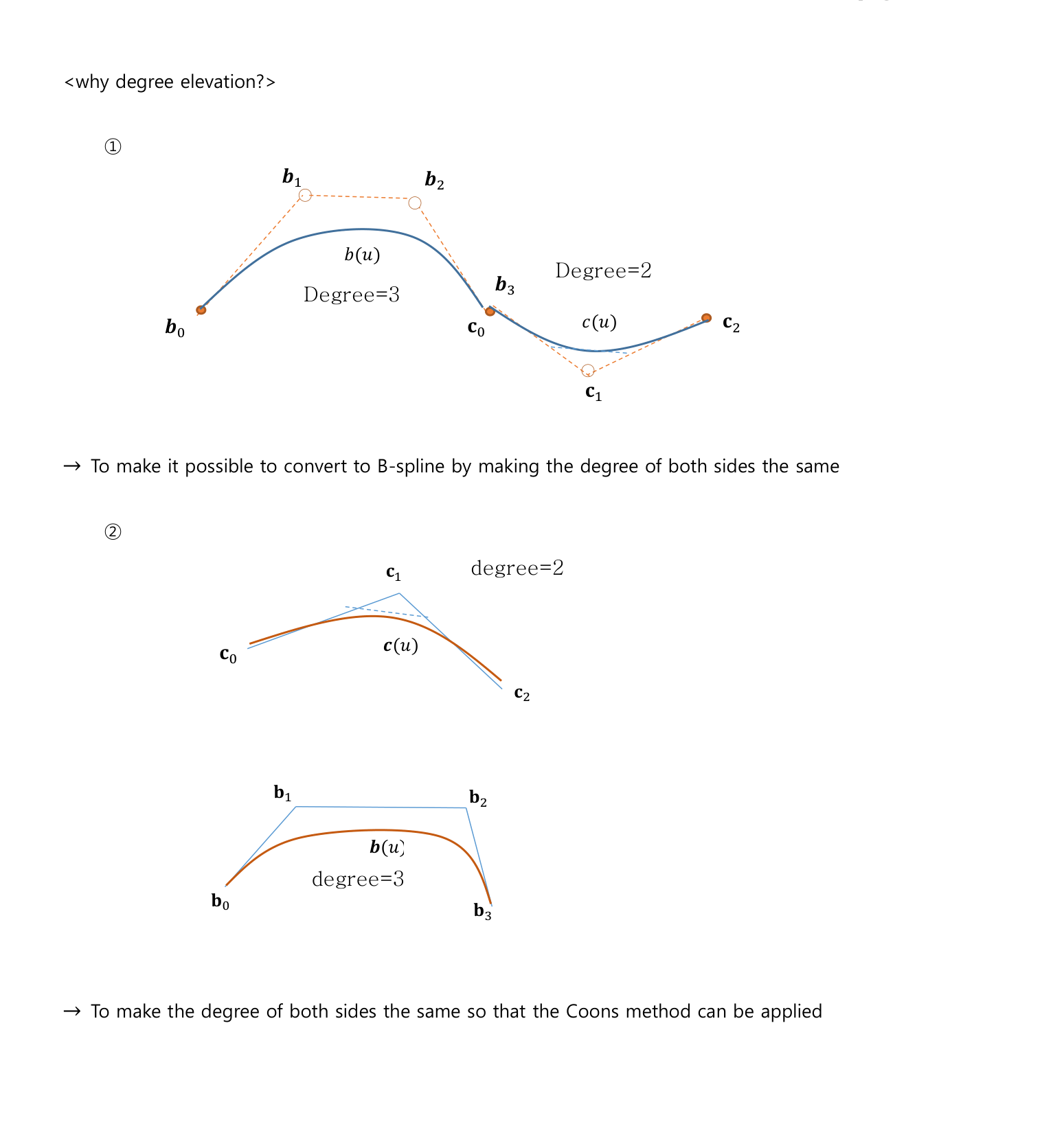
Degree elevation is used

• to make adjacent curve degrees equal before conversion to a B-spline,
• to make boundary-curve degrees equal before applying the Coons method.

9. Bézier and B-spline Surface Interpolation

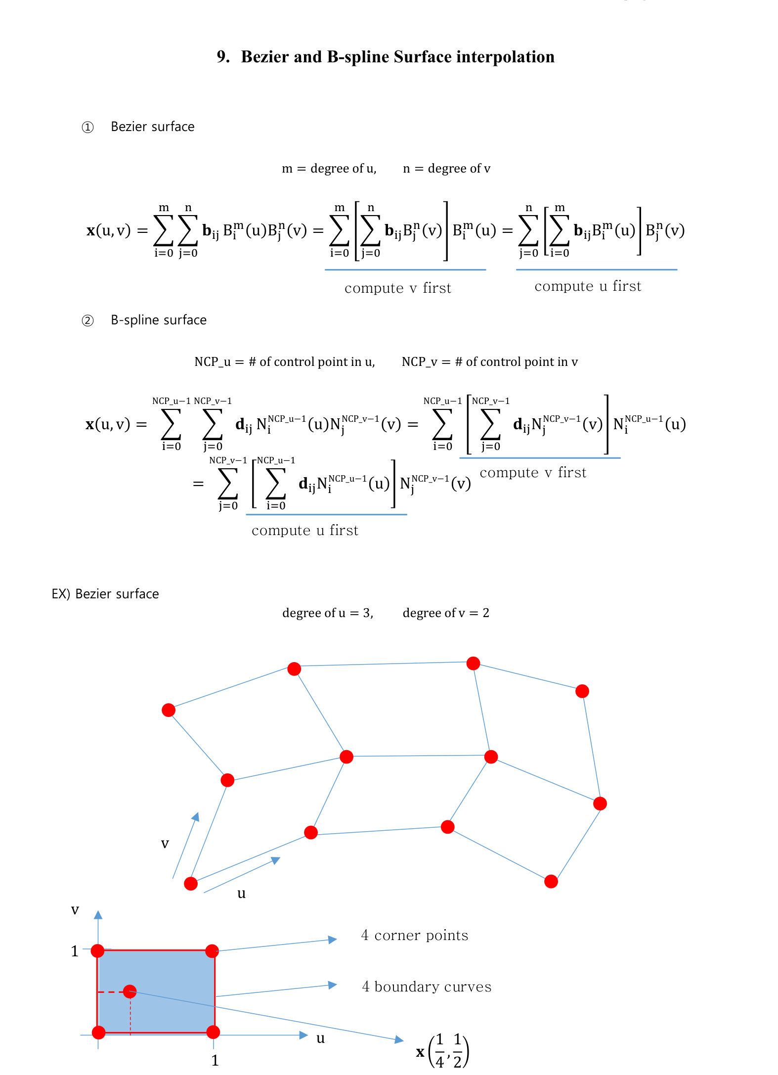
Bézier surface

\[\mathbf{x}(u,v) =\sum_{i=0}^{m}\sum_{j=0}^{n} \mathbf{b}_{ij}B_i^m(u)B_j^n(v)\]

B-spline surface

\[\mathbf{x}(u,v) =\sum_{i=0}^{NCP_u-1}\sum_{j=0}^{NCP_v-1} \mathbf{d}_{ij}N_i^{p}(u)N_j^{q}(v)\]

• Compute the $v$ direction first and then the $u$ direction.
• Or compute the $u$ direction first and then the $v$ direction.

10. B-spline Surface Interpolation

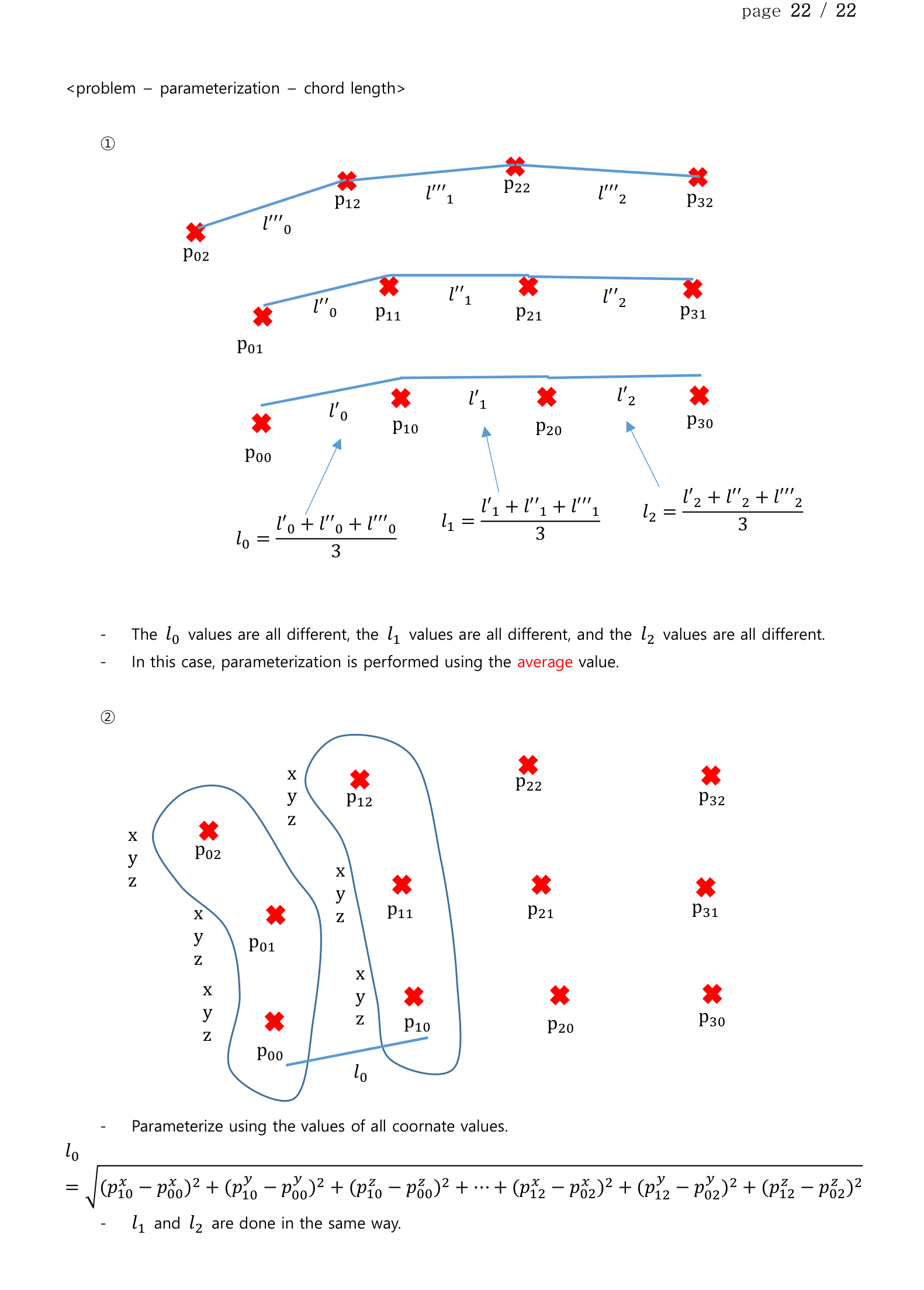
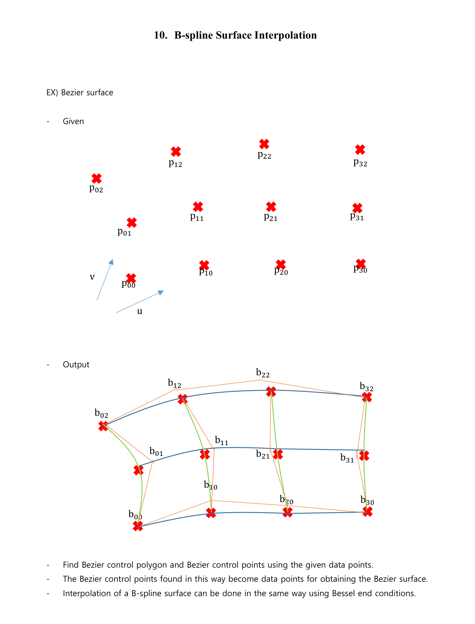
1. Parameterize each data curve.

For corresponding chord lengths from three data curves,

\[\ell_0=\frac{\ell_0'+\ell_0''+\ell_0'''}{3}\] \[\ell_1=\frac{\ell_1'+\ell_1''+\ell_1'''}{3}\] \[\ell_2=\frac{\ell_2'+\ell_2''+\ell_2'''}{3}\]

Use the mean values for parameterization.

1. Interpolate the data points in one parameter direction.
   • The control points obtained in the first direction become data points for interpolation in the second direction.
2. Interpolate in the other parameter direction.
   • B-spline surface interpolation is performed in the same way using Bessel end conditions.

Another parameterization method uses all coordinate values.

\[\ell_0 = \sqrt{ \sum_j \left[ (p_{1j}^{x}-p_{0j}^{x})^2 +(p_{1j}^{y}-p_{0j}^{y})^2 +(p_{1j}^{z}-p_{0j}^{z})^2 \right] }\]

$\ell_1$ and $\ell_2$ are obtained in the same way.