LN09. Surface Reconstruction from Offset Table

1. Surface Reconstruction from Offset Table

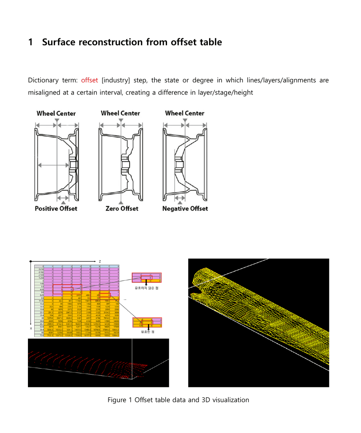
• An offset table stores points on the hull surface at each station.
• The goal is to regenerate a curved hull surface from the point data and visualize it.

Procedure

1. Read the offset-table data file.
2. Generate a winged-edge structure or an equivalent topology structure.
3. Reconstruct the surface from the offset-table points.
4. Visualize the reconstructed surface.

2. Offset Table

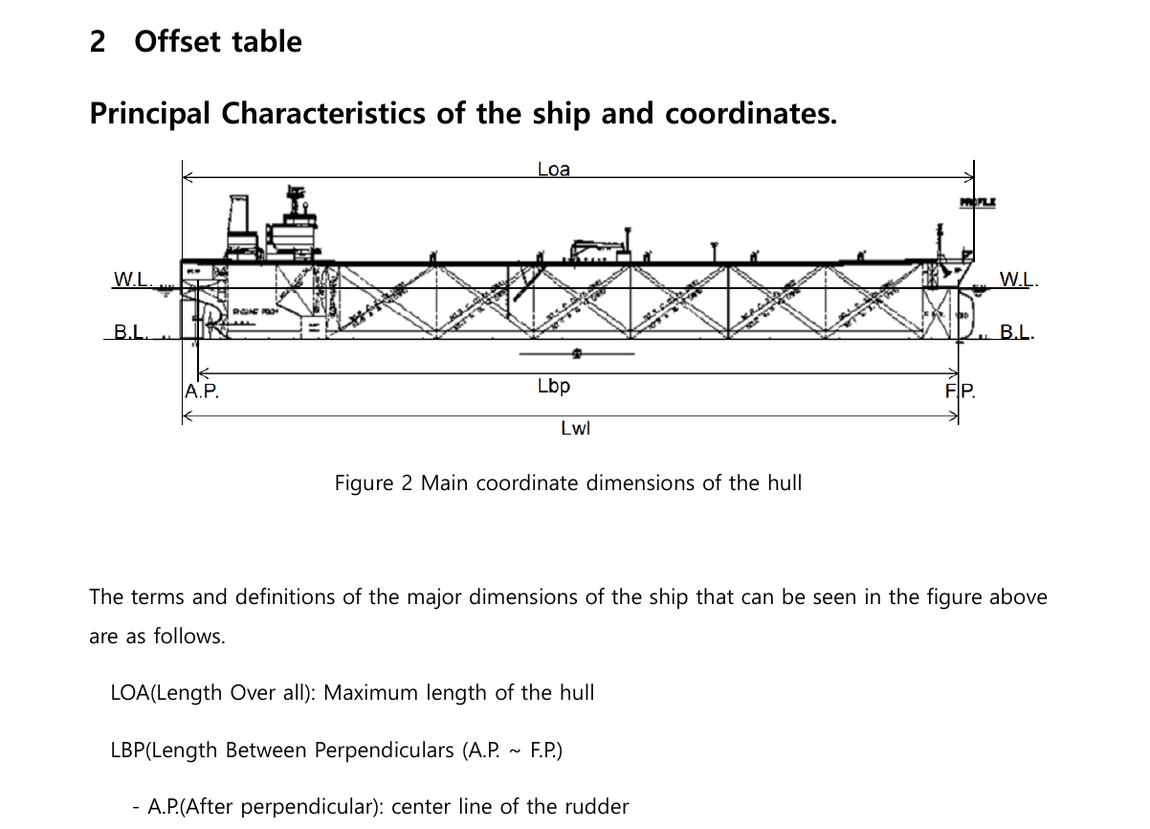
Principal Characteristics of the Ship and Coordinates

• LOA: Length Overall, the maximum length of the hull.
• LBP: Length Between Perpendiculars, from A.P. to F.P.
• A.P.: After Perpendicular, generally the center line of the rudder.
• F.P.: Fore Perpendicular, the perpendicular at the bow on the designed water line.
• W.L.: Water Line.
• B.L.: Base Line.
• The intersection of A.P. and B.L. is used as the origin.
• Use the left-hand coordinate system.

Offset-Table Data

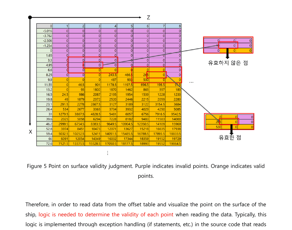
• The offset table stores point-on-surface information.
• The $X$ and $Z$ coordinates are given in meters.
• The corresponding $Y$ coordinate is stored in millimeters.

Example

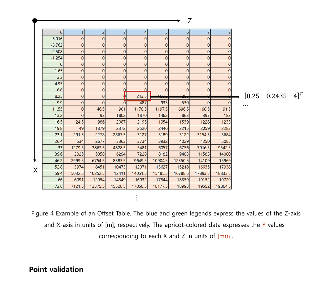
Point Validation

• A zero value does not always mean that the point is invalid.
• Examine the upper, lower, left, right, and diagonal neighboring entries.
• If at least one neighboring entry is nonzero, the point is valid.
• If every neighboring entry is zero, the point is invalid.

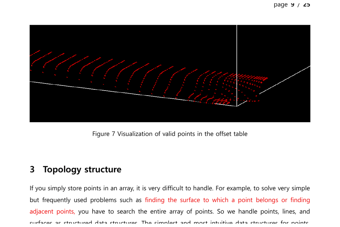
The valid points read from the table can be visualized directly before surface reconstruction.

3. Topology Structure

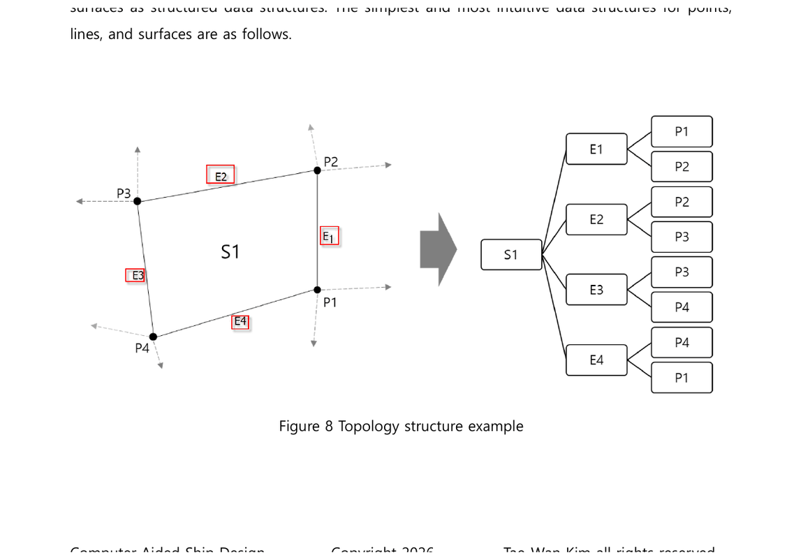
A simple array of points is inconvenient for searching adjacent points, edges, and faces. Store the geometric entities together with their adjacency information.

Winged-Edge Structure

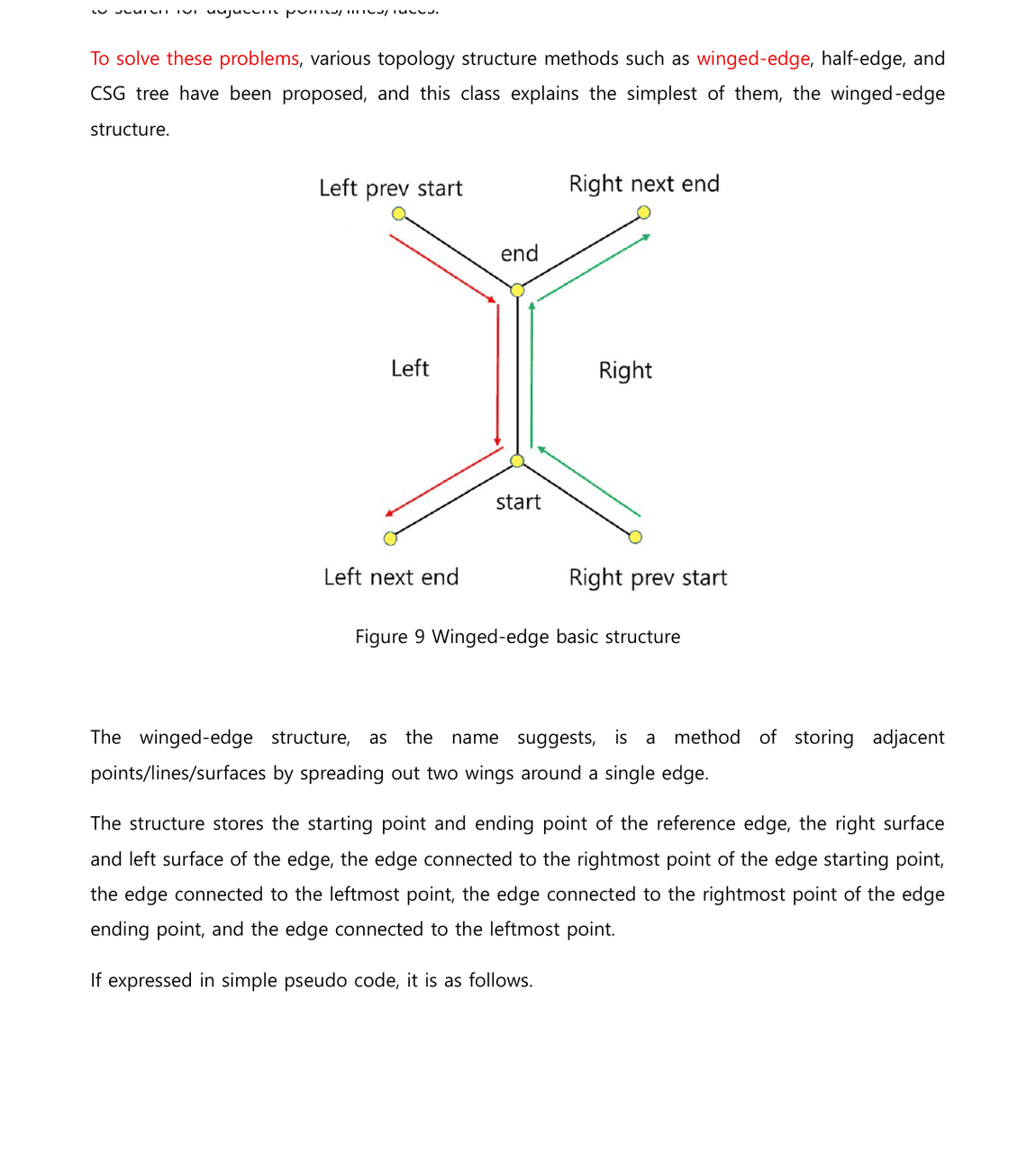
For one reference edge, store

• the start and end vertices,
• the left and right faces,
• the previous and next edges on the left face,
• the previous and next edges on the right face.

struct WingedEdge {
    Edge* self;
    Point* start;
    Point* end;

    WingedEdge* rightprev;
    WingedEdge* rightnext;
    WingedEdge* leftprev;
    WingedEdge* leftnext;

    Surface* right;
    Surface* left;
};

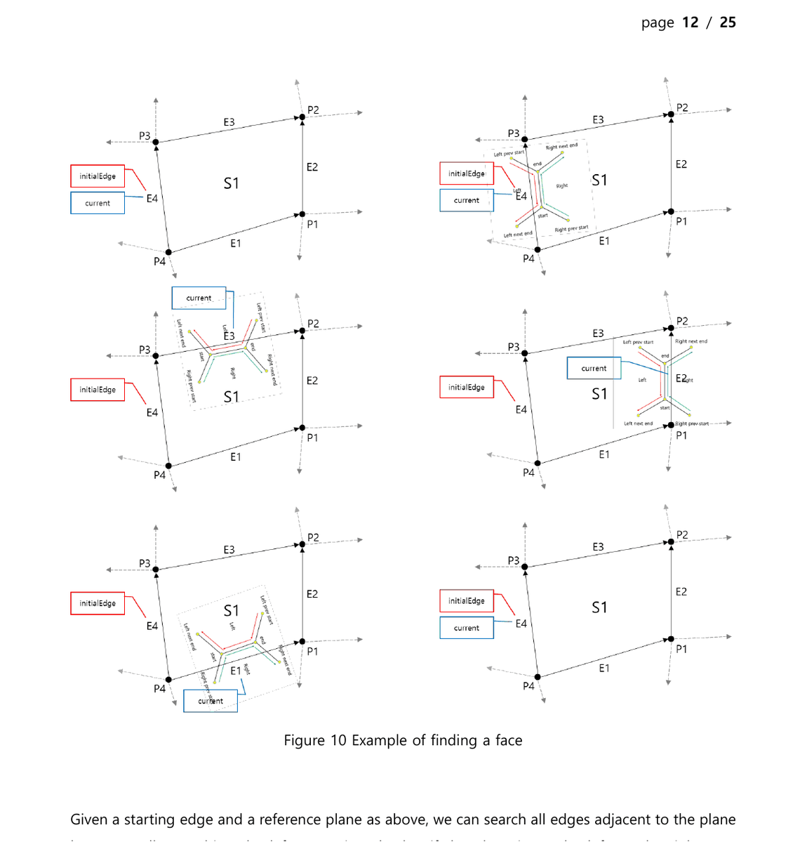
Search all edges of a face in cyclic order.

void SearchAdjacentEdgesOfSurface(WingedEdge* initial, Surface* S)
{
    WingedEdge* current = initial;

    do {
        Visit(current);

        if (current->right == S)
            current = current->rightnext;
        else
            current = current->leftnext;

    } while (current != initial);
}

4. Surface Reconstruction

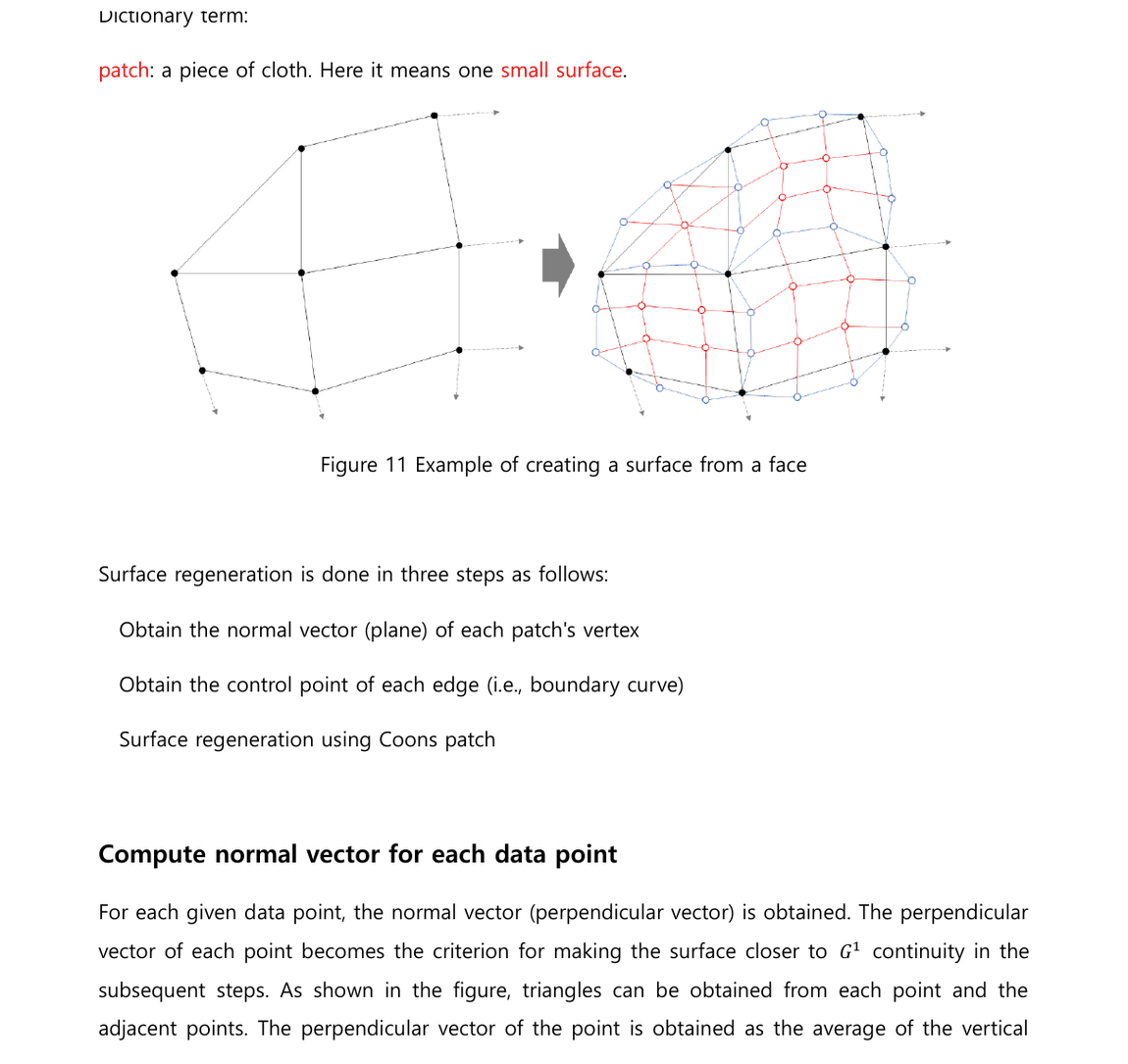
Each topology face is reconstructed as one surface patch. Adjacent patches share boundary entities, so they satisfy $C^0$ continuity automatically.

Procedure

1. Compute a normal vector at every data point.
2. Compute the control points of each boundary curve.
3. Construct a Coons patch from the boundary curves.

Compute the Normal Vector for Each Data Point

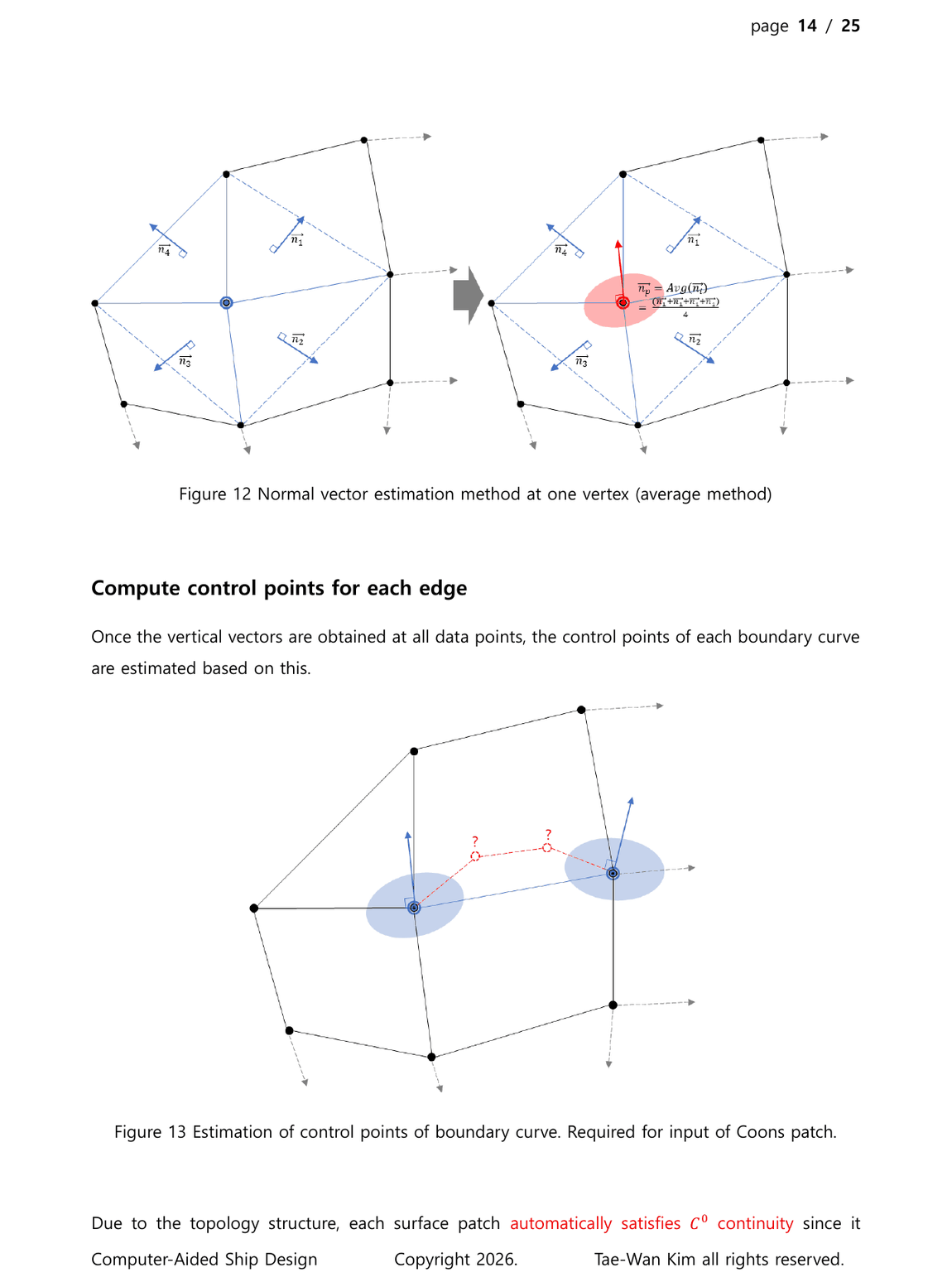
Create triangles from a vertex and its adjacent vertices. Compute the normal of each adjacent triangle and average the normals.

Compute the Control Points for Each Edge

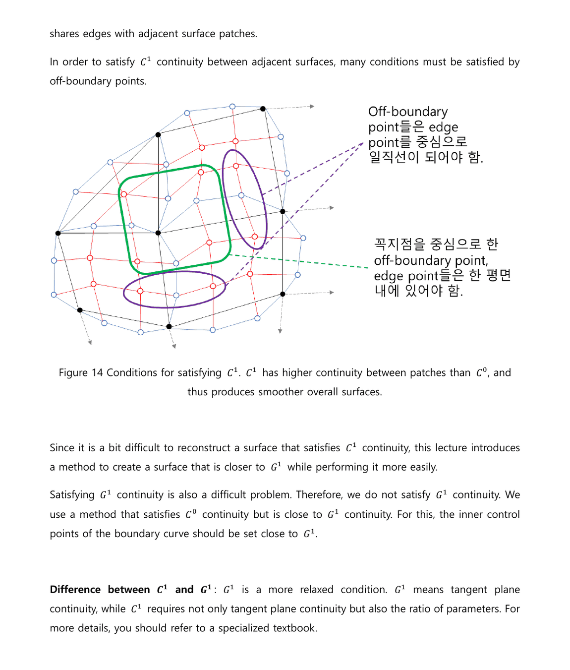
• Use the endpoint positions and endpoint normals to construct the boundary curve.
• The boundary curve is shared by the two adjacent patches.
• Exact $C^1$ continuity requires additional off-boundary constraints.
• The practical construction satisfies $C^0$ continuity and approaches $G^1$ continuity.

$G^1$ continuity is tangent-plane continuity. $C^1$ continuity additionally requires compatible parameterization across the common boundary.

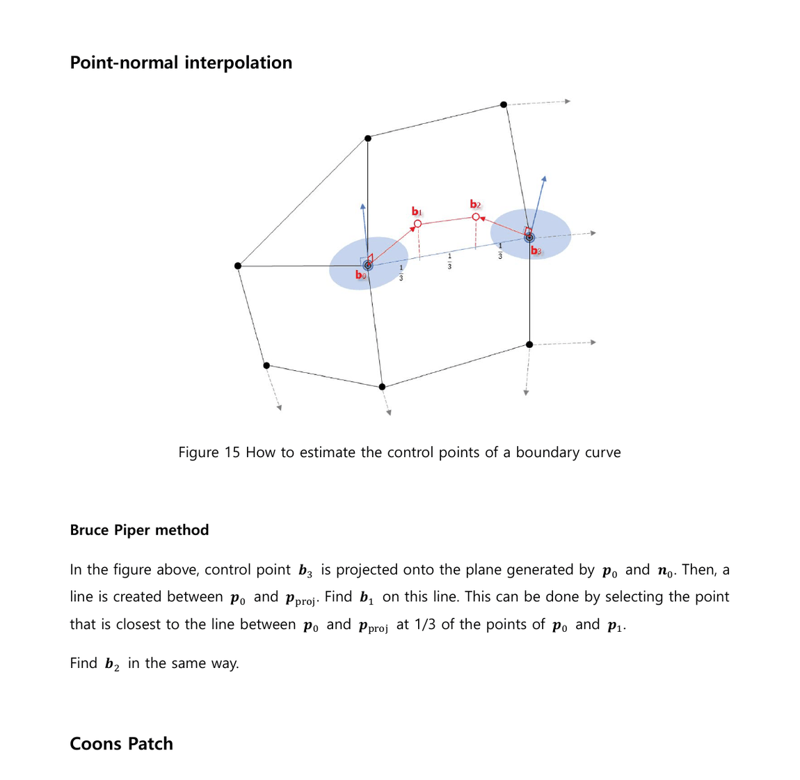
Point-Normal Interpolation

Bruce Piper method

Project the opposite endpoint onto the tangent plane at $\mathbf{p}_0$.

Place the first interior control point at one third of the projected direction.

Compute $\mathbf{b}_2$ in the same way from the other endpoint and its normal.

Coons Patch

Rectangular Coons Patch

Let $\boldsymbol{\alpha}_1(u)$ and $\boldsymbol{\alpha}_2(u)$ be the bottom and top boundaries, and let $\boldsymbol{\beta}_1(v)$ and $\boldsymbol{\beta}_2(v)$ be the left and right boundaries.

Corner compatibility

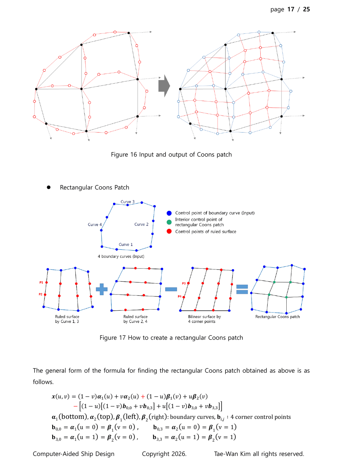
Triangular Coons Patch - Method 1

For barycentric coordinates

construct three ruled surfaces.

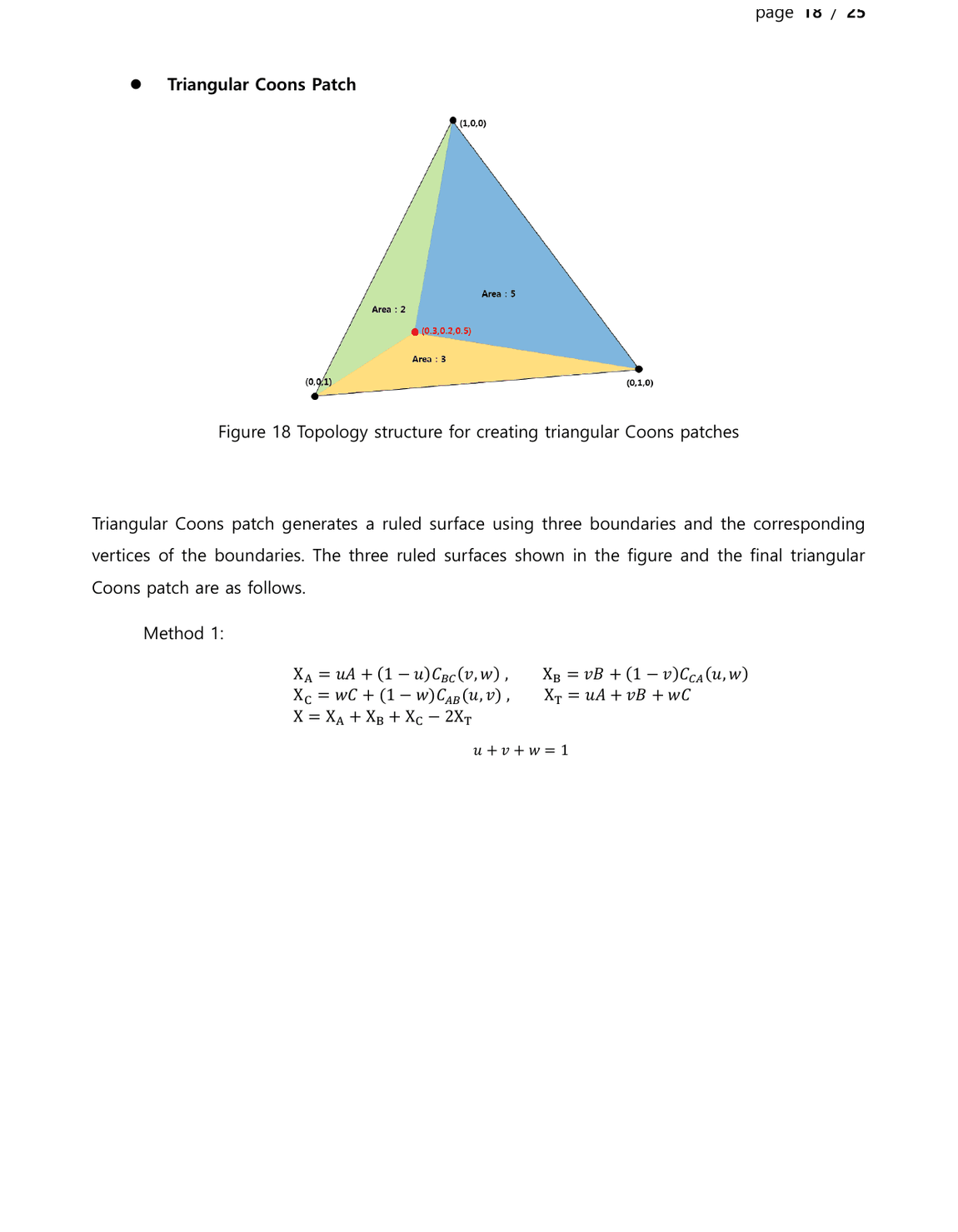
Triangular Coons Patch - Method 2

Combine the three directional patches and subtract the linear triangular patch.

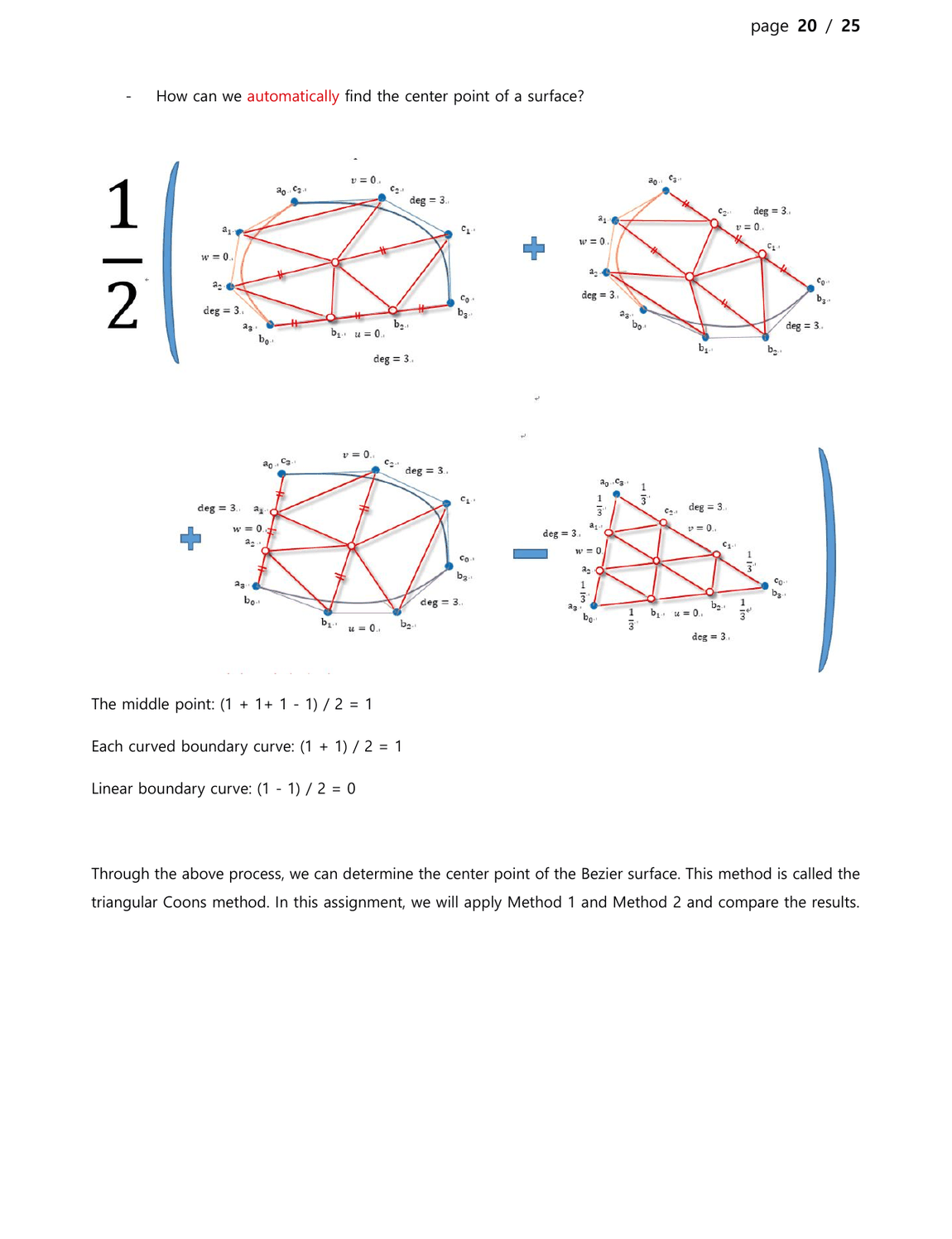
5. Visualization Using OpenGL

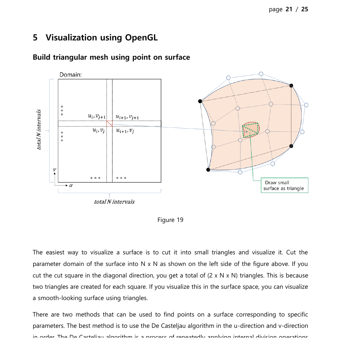
Divide the parameter domain into an $N\times N$ grid. Split every grid cell along a diagonal.

Evaluate points on the surface using the de Casteljau algorithm in one parameter direction and then in the other direction.

glBegin(GL_TRIANGLES);

for (const Triangle& tri : mesh) {
    glVertex3f(tri.p0.x, tri.p0.y, tri.p0.z);
    glVertex3f(tri.p1.x, tri.p1.y, tri.p1.z);
    glVertex3f(tri.p2.x, tri.p2.y, tri.p2.z);
}

glEnd();