[컴선설] Lec 10B Triangular Bezier Surface
LN10B. Triangular Bézier Surface
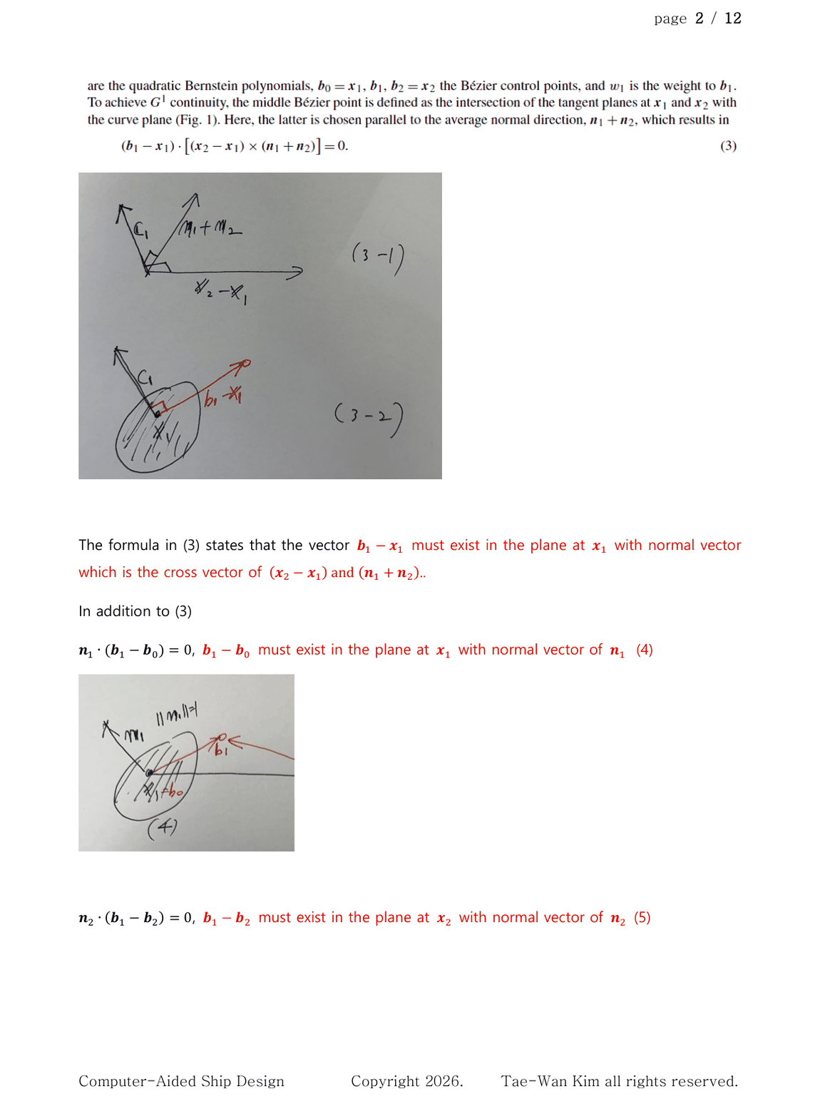
1. Boundary Curve Generation
Given
\[\mathbf{x}_{1}=\mathbf{b}_{0}, \qquad \mathbf{x}_{2}=\mathbf{b}_{2}, \qquad \mathbf{n}_{1}, \qquad \mathbf{n}_{2}\]find the middle control point $\mathbf{b}_{1}$ of a quadratic Bézier boundary curve.
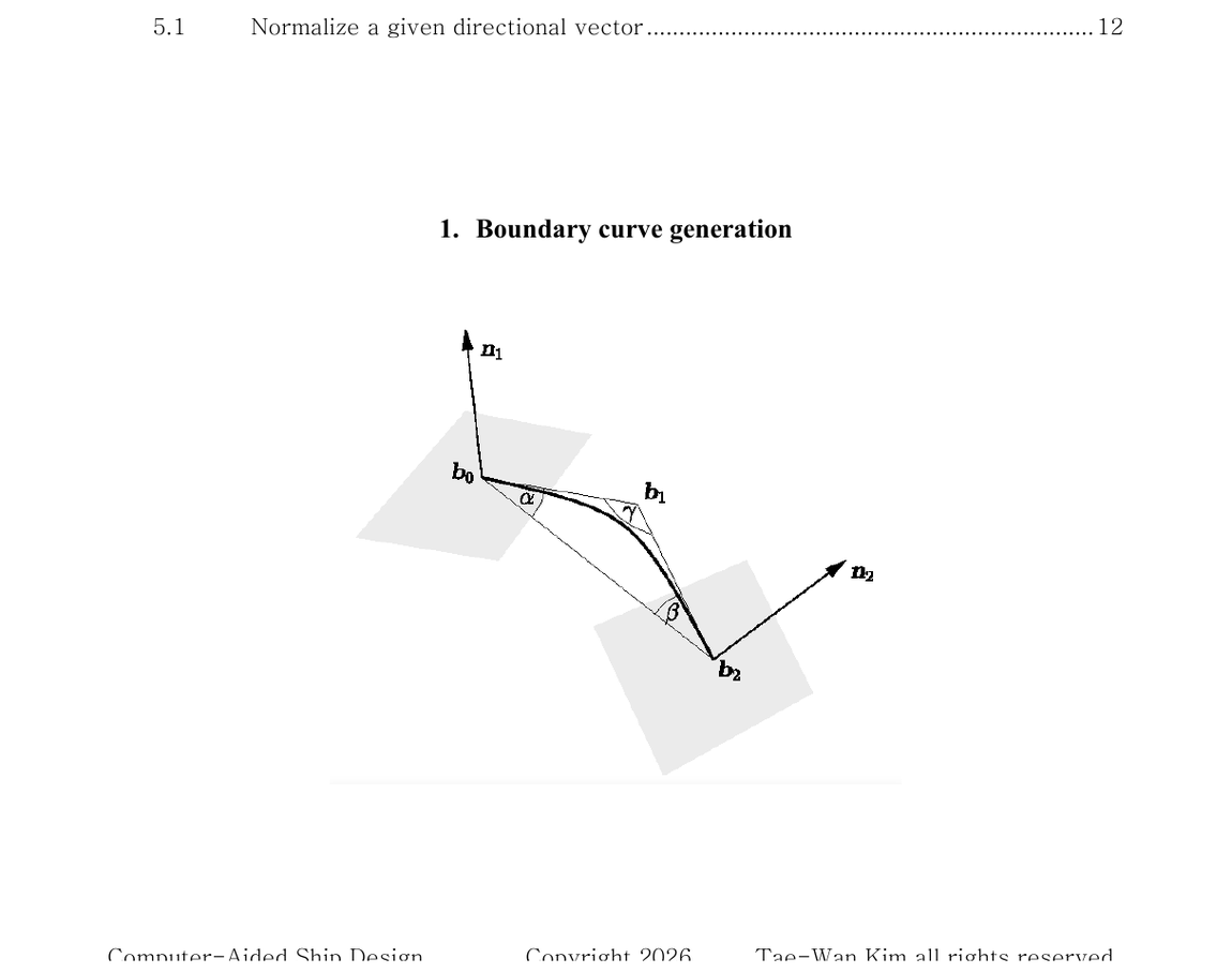
The unknown vector $\mathbf{b}_{1}$ has three scalar components. Use three plane constraints.
\[(\mathbf{b}_{1}-\mathbf{x}_{1}) \cdot \left[(\mathbf{x}_{2}-\mathbf{x}_{1})\times(\mathbf{n}_{1}+\mathbf{n}_{2})\right] =0\] \[\mathbf{n}_{1}\cdot(\mathbf{b}_{1}-\mathbf{b}_{0})=0\] \[\mathbf{n}_{2}\cdot(\mathbf{b}_{1}-\mathbf{b}_{2})=0\]Solve the three equations for
\[b_{1}^{x}, \qquad b_{1}^{y}, \qquad b_{1}^{z}\]Then elevate the quadratic boundary curve to a cubic Bézier curve.
2. Triangular Coons Patch
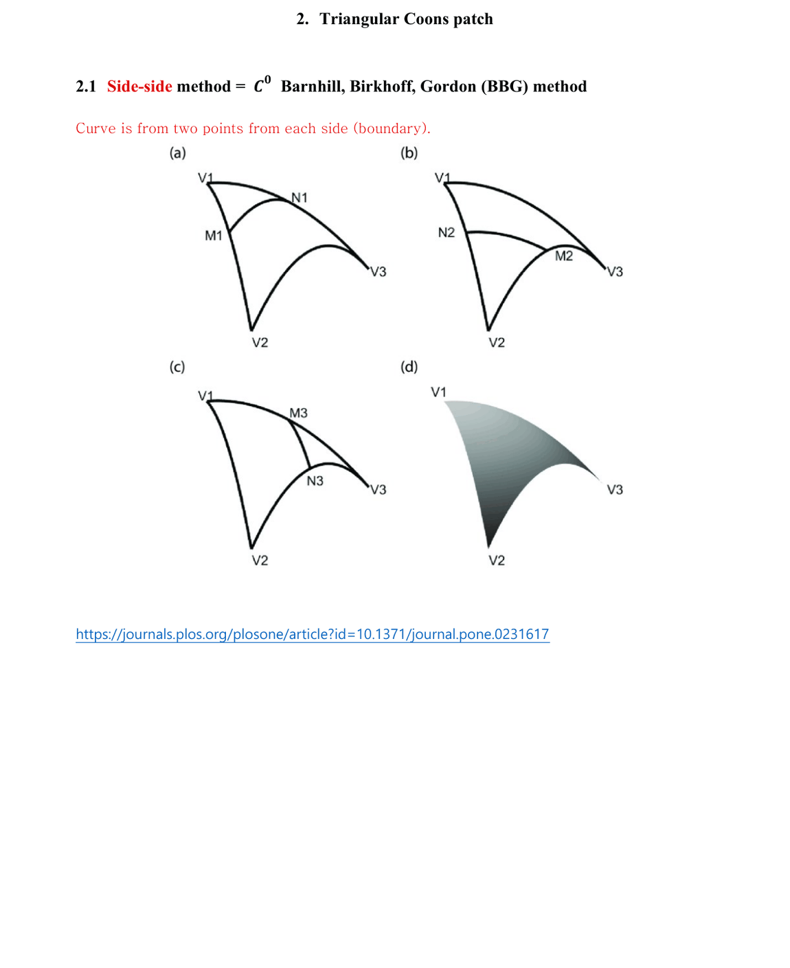
2.1 Side-Side Method - $C^0$ Barnhill, Birkhoff, Gordon Method
- A ruled surface is constructed between two boundary sides.
- The three side-side surfaces are blended to obtain the triangular patch.
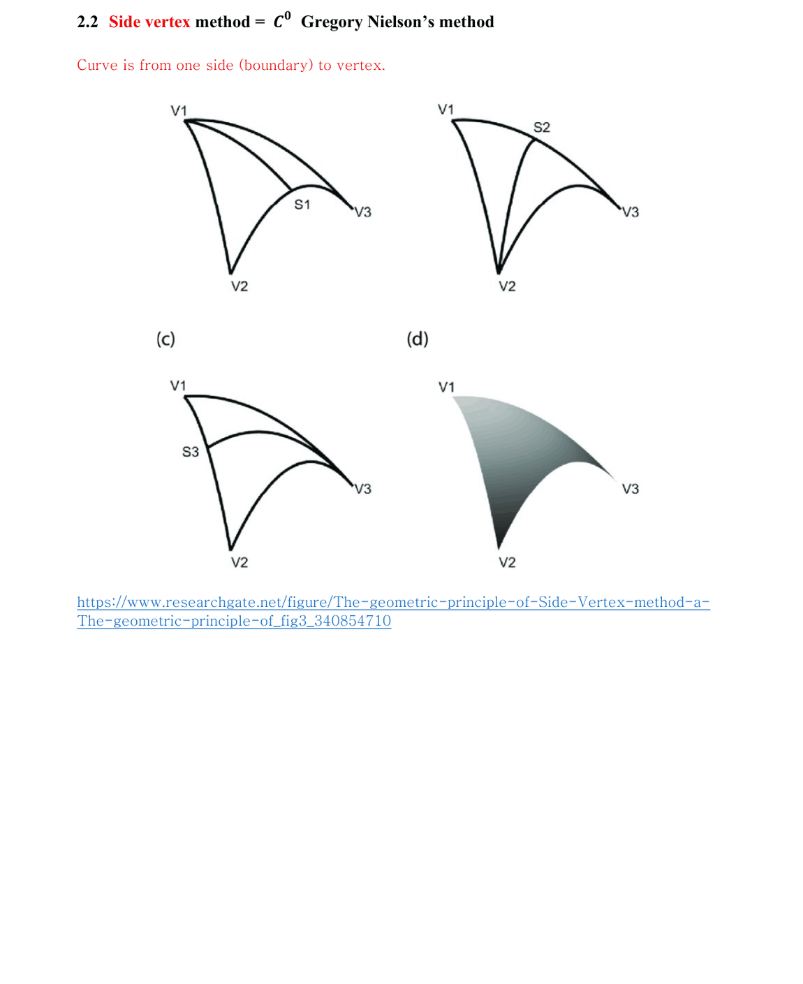
2.2 Side-Vertex Method - $C^0$ Gregory Nielson Method
- A ruled surface is constructed from one boundary side to the opposite vertex.
- Repeat the construction for all three sides.
A simple triangular Coons blend may not be as smooth as a rectangular Coons patch. Use the derivatives of the boundary curves to construct a higher-quality cubic ruled surface.
For the ruled surface associated with vertex $A$,
\[\begin{aligned} \mathbf{X}_{A} ={}&u^{3}\mathbf{A}\\ &+3\left[ \mathbf{A} +\frac{v}{3}\mathbf{T}_{AB}(1,0) +\frac{w}{3}\mathbf{T}_{AC}(1,0) \right]u^{2}(1-u)\\ &+3\left[ \mathbf{C}_{AB}(v,w) -\frac{v}{3}\mathbf{T}_{AB}(0,1) -\frac{w}{3}\mathbf{T}_{AC}(0,1) \right]u(1-u)^{2}\\ &+\mathbf{C}_{AB}(v,w) \end{aligned}\]where
\[\mathbf{T}_{AB}(u,v):\text{ derivative along }\mathbf{C}_{AB}\] \[\mathbf{T}_{AC}(u,w):\text{ derivative along }\mathbf{C}_{CA}\]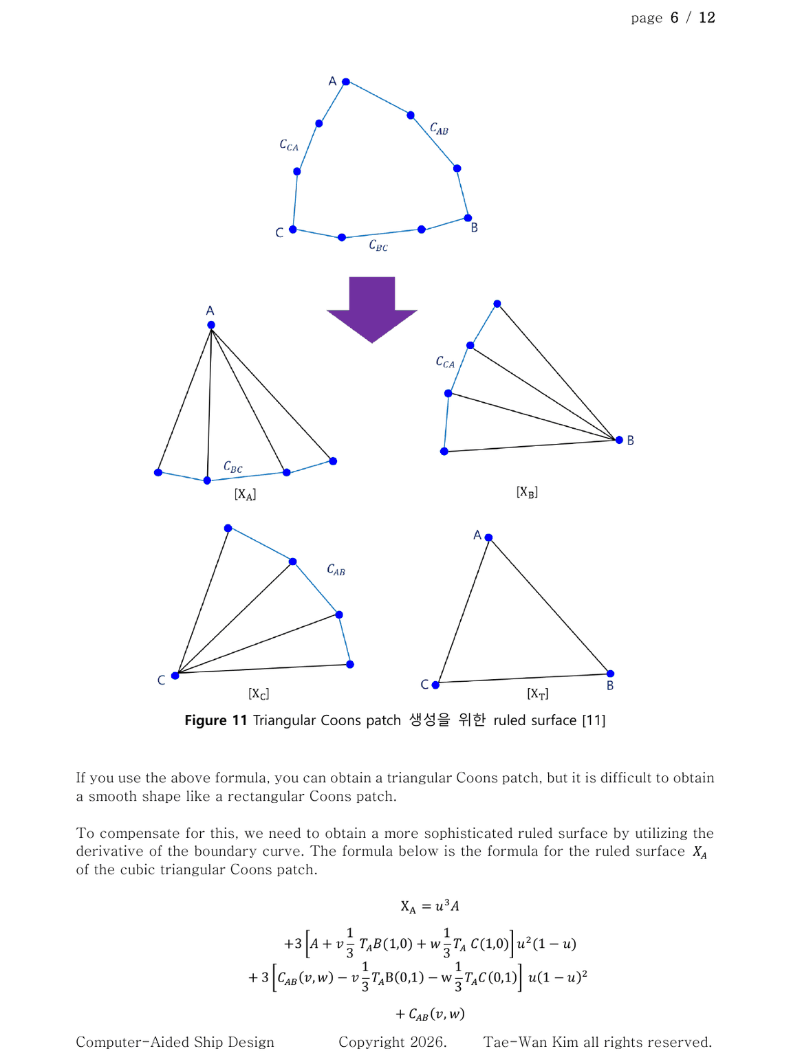
3. read_triangular_bezier_surface_data(degree_u, bez)
3.1 Data Structure of Control Points in Array Form
For a cubic triangular patch, store the control points in the following order.
| Array index | Control point |
|---|---|
b[0] |
$\mathbf{b}_{300}$ |
b[1] |
$\mathbf{b}_{210}$ |
b[2] |
$\mathbf{b}_{201}$ |
b[3] |
$\mathbf{b}_{120}$ |
b[4] |
$\mathbf{b}_{111}$ |
b[5] |
$\mathbf{b}_{102}$ |
b[6] |
$\mathbf{b}_{030}$ |
b[7] |
$\mathbf{b}_{021}$ |
b[8] |
$\mathbf{b}_{012}$ |
b[9] |
$\mathbf{b}_{003}$ |
undefined The index satisfies
\[i+j+k=n\]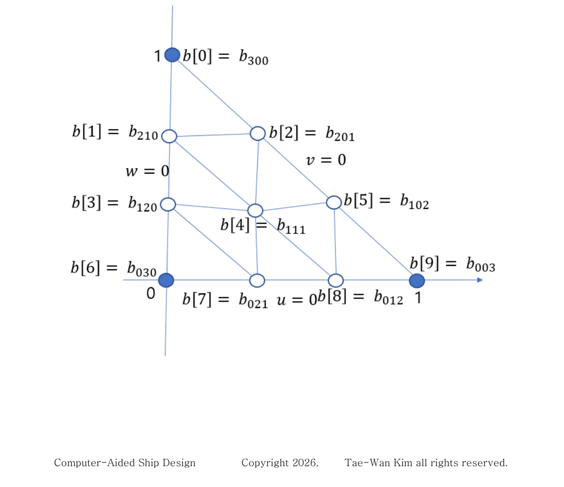
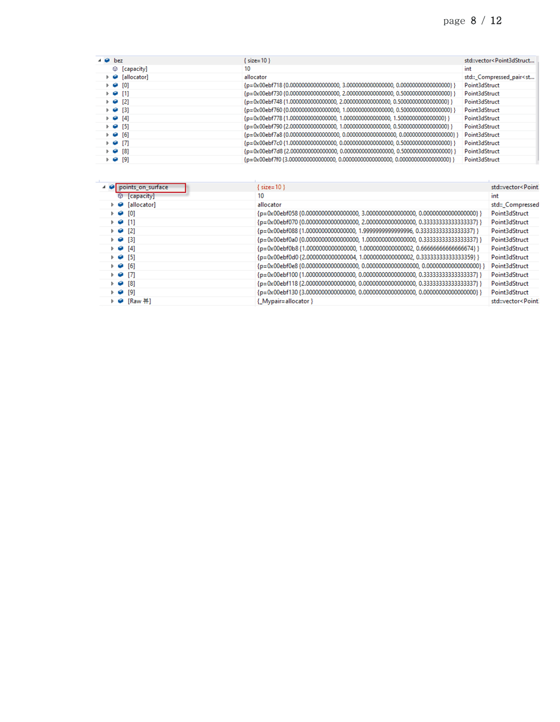
3.2 Draw Triangle Points on Surface in Array Form
For degree $n$, each row of the triangular parameter grid contains an odd number of triangles.
\[1+3+5+\cdots+(2n-1)=n^{2}\]For degree $3$,
\[1+3+5=9\]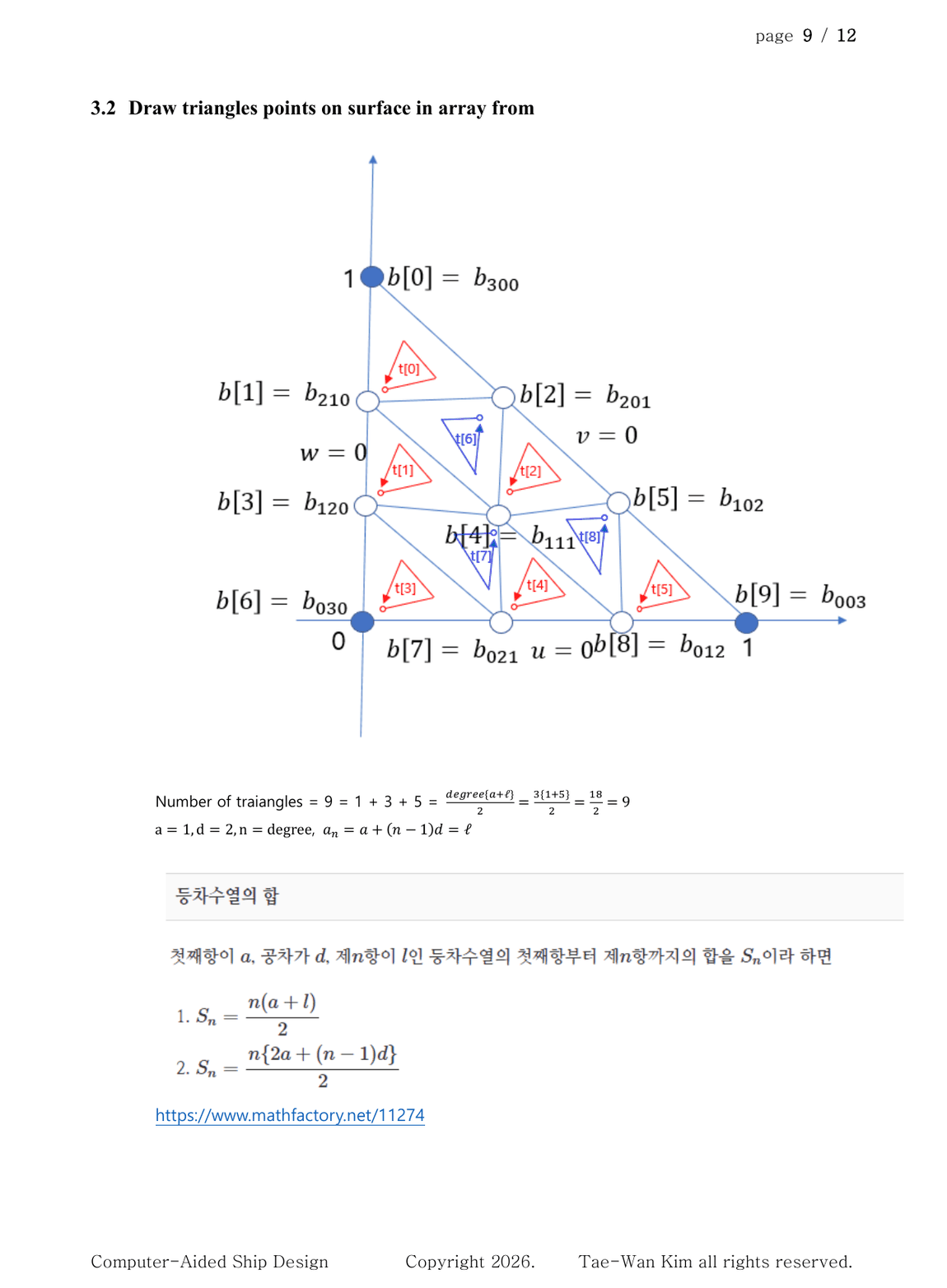
4. Draw Rectangular Coons Patch
Compute the four boundary curves, the bilinear corner patch, and the Coons blend.
Point coonsPatch(
    double u,
    double v,
    const Curve& left,
    const Curve& right,
    const Curve& bottom,
    const Curve& top)
{
    Point ruledU = (1.0 - v) * bottom(u) + v * top(u);
    Point ruledV = (1.0 - u) * left(v) + u * right(v);

    Point bilinear =
        (1.0 - u) * (1.0 - v) * bottom(0.0)
        + u * (1.0 - v) * bottom(1.0)
        + (1.0 - u) * v * top(0.0)
        + u * v * top(1.0);

    return ruledU + ruledV - bilinear;
}
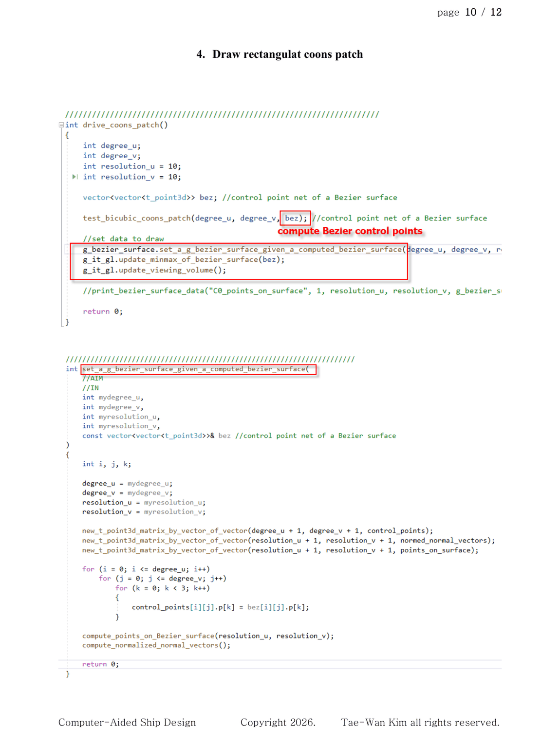
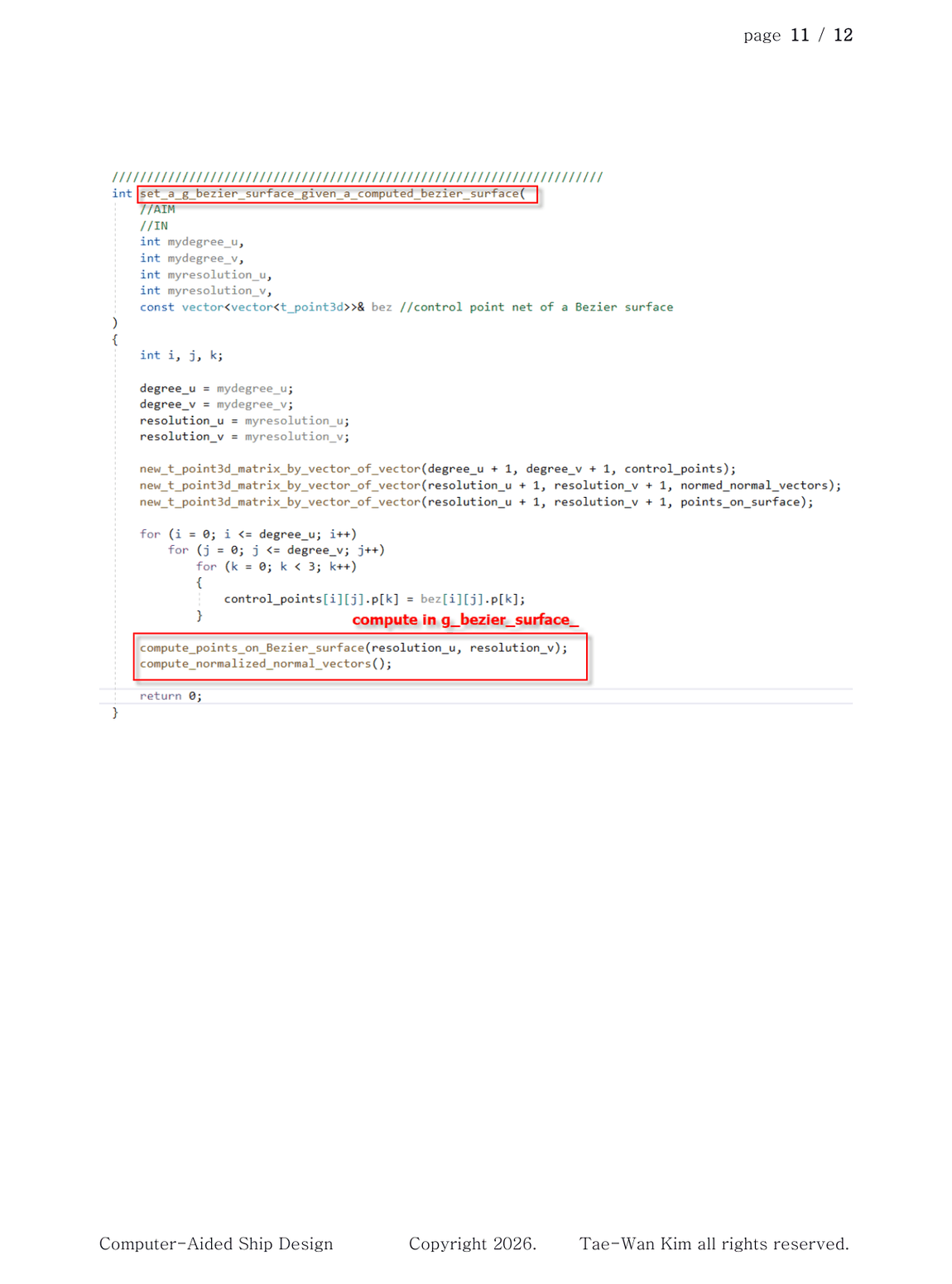
Generate the points on the patch over the parameter grid and use them as the vertices of the visualization mesh.
5. Directional Derivative of a Triangular Bézier Surface
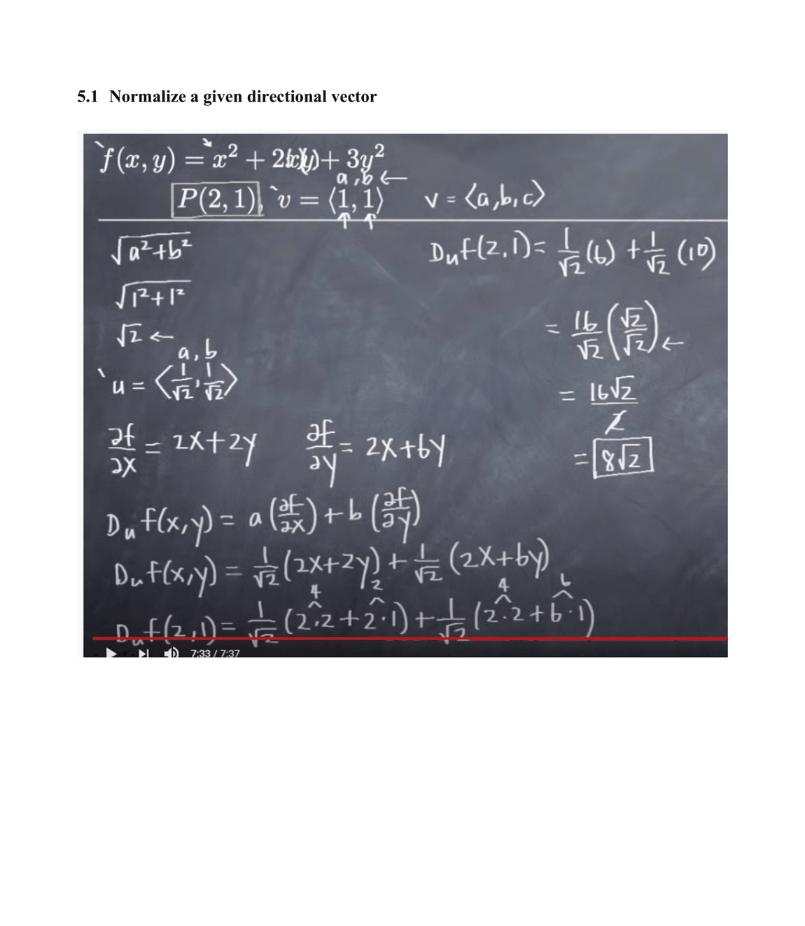
5.1 Normalize a Given Directional Vector
For a direction vector
\[\mathbf{v}=\langle a,b\rangle\]use the unit vector
\[\mathbf{u} = \frac{\mathbf{v}}{\|\mathbf{v}\|} = \left\langle \frac{a}{\sqrt{a^{2}+b^{2}}}, \frac{b}{\sqrt{a^{2}+b^{2}}} \right\rangle\]The directional derivative is
\[D_{\mathbf{u}}f = \nabla f\cdot\mathbf{u}\]Example
\[f(x,y)=x^{2}+2xy+3y^{2}\] \[\nabla f = \left\langle 2x+2y, 2x+6y \right\rangle\]At $P=(2,1)$ in the direction $\mathbf{v}=\langle1,1\rangle$,
\[\mathbf{u} = \left\langle \frac{1}{\sqrt{2}}, \frac{1}{\sqrt{2}} \right\rangle\] \[D_{\mathbf{u}}f(2,1) = \frac{6}{\sqrt{2}} + \frac{10}{\sqrt{2}} = 8\sqrt{2}\]For a parametric surface, compute two independent directional derivatives and take their cross product to obtain the normal vector.