[PSA] Chapter 10 - Power Flow Analysis

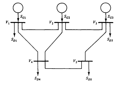
• System one-line diagram

10.1 Power Flow Equations

\[S_i \triangleq S_{Gi}- S_{Di} = \sum_{k=1}^n S_{ik}\]

• Generating / Draining : Effective power injected to the transmission system
• We can also define bus current $I_i$ which is total $a$ current entering the transmission system

\[I_i = I_{Gi}-I_{Di} = \sum_{k=1}^n I_{ik}\]

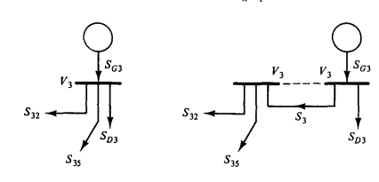
• With bus admittance matrix, we can calculate power of $i$th bus

\[\begin{aligned}S_i&=V_i I_i^*\\&=V_i\left(\sum_{k=1}^{n}Y_{ik}V_k\right)^*\\&=V_i\sum_{k=1}^{n}Y_{ik}^{*}V_k^{*}\qquad i=1,2,\ldots,n\end{aligned}\tag{10.3}\] \[\begin{aligned}V_i&\triangleq|V_i|e^{j\angle V_i}=|V_i|e^{j\theta_i}\\\theta_{ik}&\triangleq\theta_i-\theta_k\\Y_{ik}&\triangleq G_{ik}+jB_{ik}\end{aligned}\]

We can set complex voltages and admittances where

$G$ : conductance, $B$ : susceptance

\[\begin{aligned}S_i&=\sum_{k=1}^{n}|V_i||V_k|e^{j\theta_{ik}}(G_{ik}-jB_{ik})\\&=\sum_{k=1}^{n}|V_i||V_k|(\cos\theta_{ik}+j\sin\theta_{ik})(G_{ik}-jB_{ik})\qquad i=1,2,\ldots,n\end{aligned}\tag{10.4}\] \[\begin{aligned}P_i&=\sum_{k=1}^{n}|V_i||V_k|(G_{ik}\cos\theta_{ik}+B_{ik}\sin\theta_{ik})\\Q_i&=\sum_{k=1}^{n}|V_i||V_k|(G_{ik}\sin\theta_{ik}-B_{ik}\cos\theta_{ik})\end{aligned}\tag{10.5}\]

We can calculate $P$, $Q$ from network

10.2 The Power Flow Problem

• Generator buses : supplied by generators
• Load buses : buses without generators

Power flow problem

• Given two variables for each bus, figure the rest two ($P_i, Q_i, \vert V_i \vert, \theta_i$)

Slack bus (Swing bus)

• Normally choose Bus 1 as a slack bus
• Given $\vert V_1 \vert, \theta_1$ / Figure $P_1, Q_1$, $\theta_1 = 0$
• Slack bus provides transmission loss, mismatch between generation and load, reactive-power mismatch (provides norm)
• Slack bus compensates transmission loss and error, does not designate $P_1 $ before determining every values
• Slack bus’s angle becomes norm

PV bus or voltage-control bus

\[\text{PV bus:}\qquad P_i,\ |V_i|\ \text{given},\qquad Q_i,\ \theta_i\ \text{unknown}\]

• Controls $P_i$ with turbine or governor input
• Controls $\vert V_i \vert$ with excitation system
• Determines $Q_i$ with power-flow solution

PQ bus or load bus

\[\text{PQ bus:}\qquad P_i,\ Q_i\ \text{given},\qquad|V_i|,\ \theta_i\ \text{unknown}\]

Generator reactive-power limit

\[Q_i^{\min}\le Q_i\le Q_i^{\max}\]

• Reactive power limit exists on real generators
• If $Q_i$ reaches the limit, it fixes reactive power value to maximum and converted into PQ bus
• PV bus → PQ bus

Constant-impedance load

• If load is given with impedance $Z_{Di}$ not complex power, Convert to admittance by taking reciprocal
• Setting Complex power to zero, add admittance to diagonal term of bus admittance matrix

\[Y_{ii}^{(\mathrm{new})}=Y_{ii}+Y_{Di}, \qquad S_{Di} = 0\]

Existance and uniqueness of solution

• If two solutions exists, normally High-voltage solution is answer. Not typical driving point for low-voltage

10.3~10.6 Numerical iteration Methodologies

10.7 Decoupled Power Flow

• Typicial properties of standard transmission system
  1. Transmission line is inductive : $|G_{ik}|\ll|B_{ik}|$
  2. Small angle difference when standard operation : $\vert \theta_i - \theta_k \vert \ll 1$
  3. Flat voltage profile : $\vert V_i \vert \approx 1 \text{p.u.}$
• At this condition, $P - \theta$ coupled, $Q-\vert V\vert$ coupled.
• Therefore, ${\bf J}_{12} \approx 0, {\bf J}_{21} \approx 0$ for jacobian matrix descring coupled equation

Decoupled Newton-Raphson

\[\begin{bmatrix} \Delta\mathbf P\\ \Delta\mathbf Q \end{bmatrix} = \begin{bmatrix} \mathbf J_{11}&\mathbf J_{12}\\ \mathbf J_{21}&\mathbf J_{22} \end{bmatrix} \begin{bmatrix} \Delta\boldsymbol\theta\\ \Delta|\mathbf V| \end{bmatrix}\]

• Coupled equation can be seperated by following

\[\mathbf J_{11} \Delta\boldsymbol\theta = \Delta\mathbf P \tag{10.51a}\] \[\mathbf J_{22} \Delta|\mathbf V| = \Delta\mathbf Q \tag{10.51b}\]

Fast-decoupled power flow

• Additionally we can approximate Jacobian into susceptance of $Y_{bus}$ if we assume flat-voltage, small-angle approximation

\[-\mathbf B\Delta\boldsymbol\theta = [\mathbf V]^{-1}\Delta\mathbf P \tag{10.58a}\] \[-\mathbf B\Delta|\mathbf V| = [\mathbf V]^{-1}\Delta\mathbf Q \tag{10.58b}\]

Where $ \mathbf B=\Im{\mathbf Y_{\mathrm{bus}}}_{\mathrm{reduced}} $

• $\bf B$ is constant over iteration → No need to re-calculate Jacobian every iteration

10.8 Control Implications

• For small perturbations, inverse of the Jacobian works well

Line Loss

• Total active power loss can be figured with net bus injections
• Active power loss of each line $i-k$

\[P_{\mathrm{loss},ik} = \frac{r_{ik}}{|z_{ik}|^2} \left( |V_i|^2+|V_k|^2 -2|V_i||V_k|\cos\theta_{ik} \right)\]

• Implies if generation is near loss, it can reduce line current and loss.

10.9 Regulating Transformers in Power Flow

• Tap ratio or phase shift appears in equation directly

1. Voltage-magnitude regulating transformer

\[\begin{bmatrix} I_1\\ I_2 \end{bmatrix} = \begin{bmatrix} y&-\dfrac{y}{n}\\[2mm] -\dfrac{y}{n}&\dfrac{y}{n^2} \end{bmatrix} \begin{bmatrix} V_1\\ V_2 \end{bmatrix}\]

• by changing tap $n$, Three terms vary
• Two ways of including transformer into power flow
  1. Assign $n=1/a$ as a given parameter : Treat Controlled bus as normal PQ bus / Calculate for $\vert V \vert$ and $\theta$
  2. Assign Controlled-bus voltage $\vert V \vert$ : $n $ is a new variable. Add rows and columns for jacobian
• Second method expresses automatic tap-changing transformer

2. Phase-shifting transformer

\[\begin{bmatrix} I_1\\ I_2 \end{bmatrix} = \begin{bmatrix} y&-ye^{-j\phi}\\ -ye^{j\phi}&y \end{bmatrix} \begin{bmatrix} V_1\\ V_2 \end{bmatrix}\]

• Magnitude ratio : $1$, phase shift : $\phi$
• If phase shifter is included, there no needs for $Y_{bus}$ to be symmetric

10.10 Power Flow for Large Power Systems

• Sparsity : Jacobian and $Y_{bus}$ are sparse
• LU factorization and fill-in : new non-zero term can be created (so-called fill-in)